Walkthrough on filament models

This walkthrough is a step-by-step guide that teaches how to extract subtomograms from filament-like structures using the Dynamo filament models.

Data

We are going to demonstrate the basic ideas and tools on a synthetic dataset. This data is already available in the catalogue manager. It can be accessed by first opening the catalogue manager using the command:

dcm

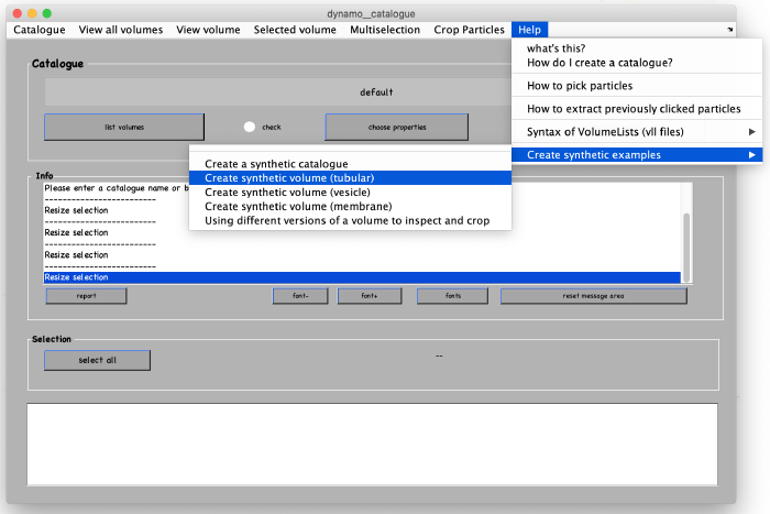
After the catalogue manager opens, we create the synthetic tomogram that includes tubular looking objects (filaments) in the following way:

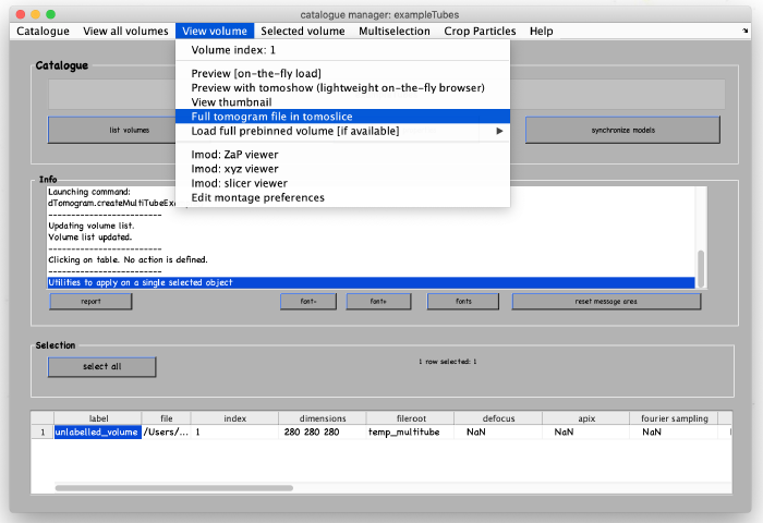
A new tomogram entry appears in the catalogue manager. Any further annotations (models) to the tomogram will be linked to this entry. Select the entry and open it:

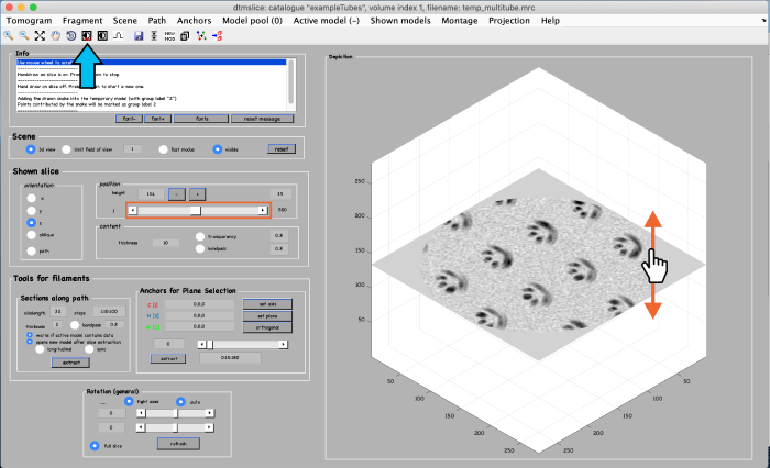
A tomogram viewer opens. You might need to adjust the contrast (blue arrow). To move through the tomogram slices, you can either use the mouse wheel, click and drag the tomogram slice up and down (orange arrows), or move the position control left and right (orange box).

Manual annotation

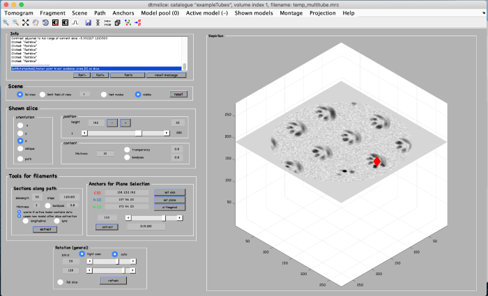
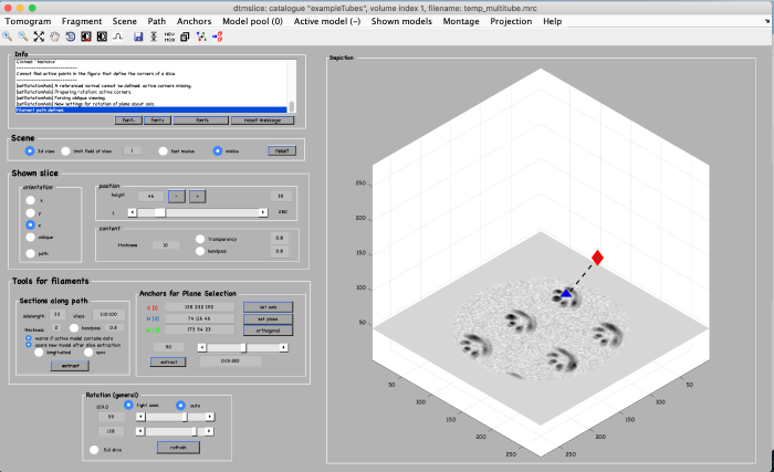
To be able to later annotate a filament of interest, we first create an alternative view by using the anchor points. We start by marking the beginning of a filament. Move the slice up to a high z height. Place the mouse in the center of a filament and press the key [1] on the keyboard to place an anchor in the beginning of the filament. Note: to correct the anchor point just click the [1] key again.

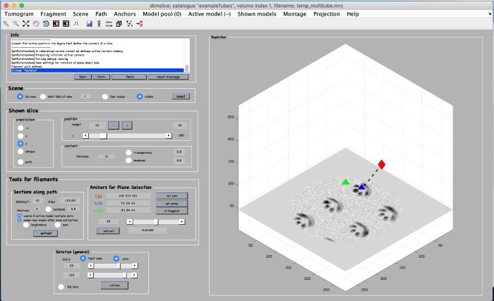
To mark the end of the filament, move to a low z-height. Place the mouse in the center of the same filament and press the key [2] on the keyboard to place the anchor in the end of the filament.

Finally, a third anchor point (key [3]) is placed to define the width of the alternative view that we are creating:

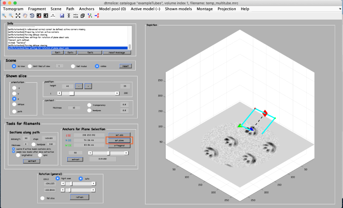
Click on set plane (orange box) to define a plane along the anchor points:

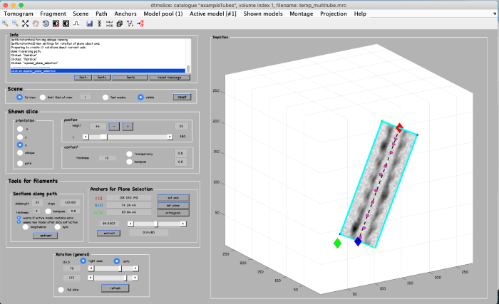
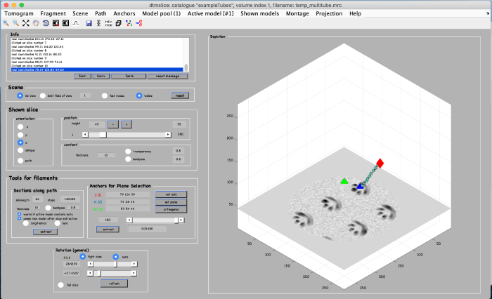
Use the anchor for plane selection control (orange box) to activate and rotate the viewing plane around the filament:

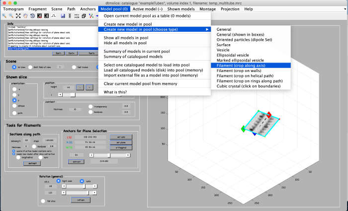
Annotations are done within a so called model. We open a new model of type filament as follows:

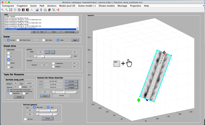
If necessary, click and drag while holding the control key to rotate the view of the tomogram to get a good view of the filament:

To add annotation points to the model, place the mouse on the filament and press the key [c]. Use the right-click to delete points if needed. Note: A known bug may cause the clicked points to be generated slightly displaced from the mouse cursor. Maximize the window of the tomogram viewer to get rid of this effect. Generate about 10 points:

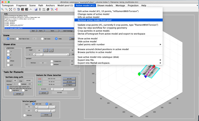
We show you an alternative way to click the points on the filament. To demonstrate this, we first delete the current points as shown below:

We create a new model in the same way as before:

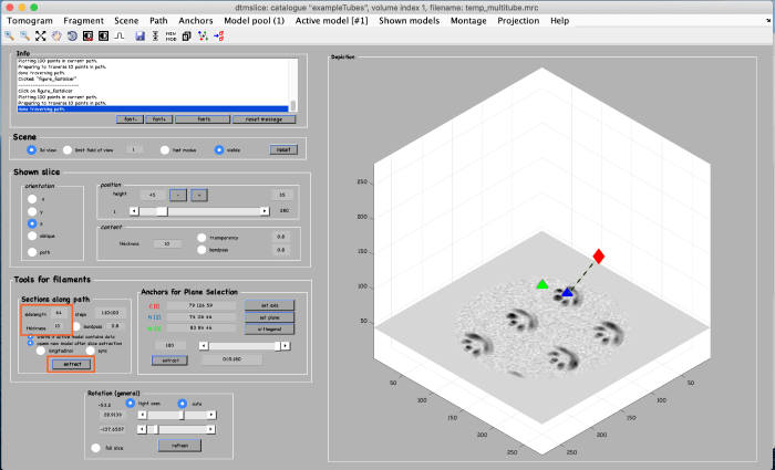
For this alternative method, we first create a view of orthogonal slices through the filament. In tools for filaments set sidelength to 64 and thickness to 10 (see orange box). Then click on extract (see orange box):

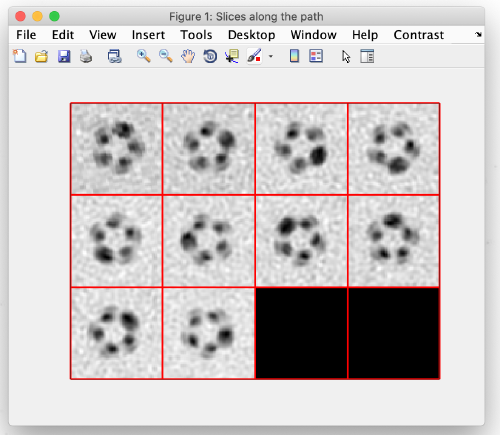
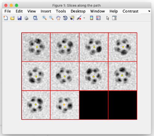
You get a new window with the view of the orthogonal slices through the filament:

Same as before, using the [c] key, add model points at the center of the tube filament:

When done, close the window and you should see your clicked points in the main view:

Generate subtomogram coordinates

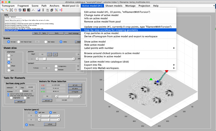
Using the clicked model we can now define the coordinates where the subvolumes will be extracted. To do that, we first processes the clicked model points using the model workflow to generate a user specific cropping geometry. Open the workflow:

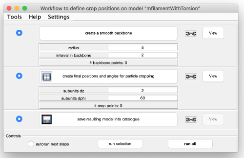
You get a new window with the model workflow. It has three large buttons (and corresponding input parameters below) that are executed sequentially starting from top. Click on create a smooth backbone:

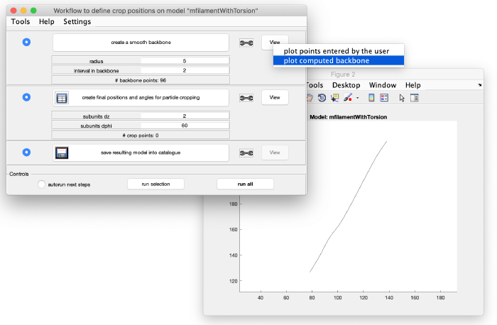
This creates an interpolation through the points in the model. Visualize it by left-clicking on view:

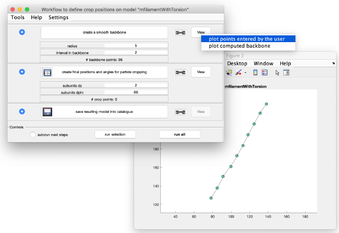
Add the clicked model points to the graph:

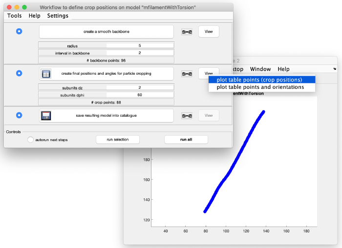
This looks good. We now create coordinates along this interpolation (backbone) which will be used as centers for the subtomogram extraction (cropping). Click on create final positions and angles for particle cropping. Ignore the angles, as they are not part of this model. Visualize the crop positions:

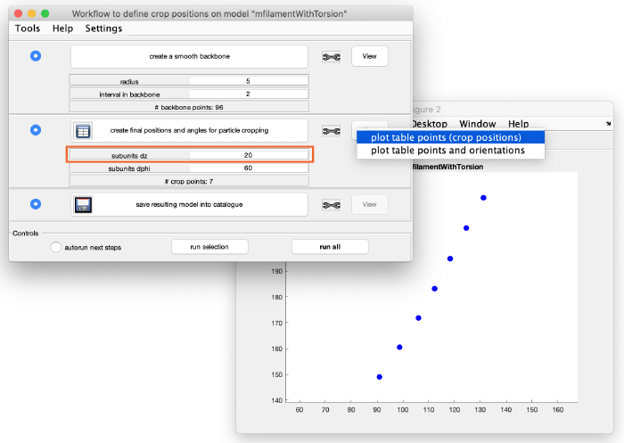
You can see that these are too many crop points. Adjust the spacing between the cropping points by changing the parameter subunits dz from 2 to 20 (see orange box). Click again create final positions and angles for particle cropping to update the information and visualize the new crop points:

This looks much better. Save the model by clicking on save resulting model into catalogue and we can move to the subtomogram extraction.

Extract subtomograms

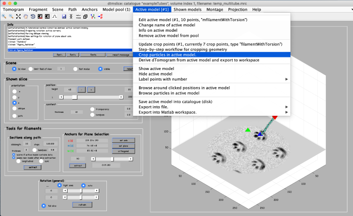
In this final step we extract subvolumes at the coordinates defined before. First, open the partcile extraction GUI:

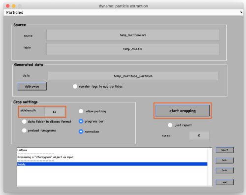
Set the sidelength to 64 and click on start cropping (orange box):

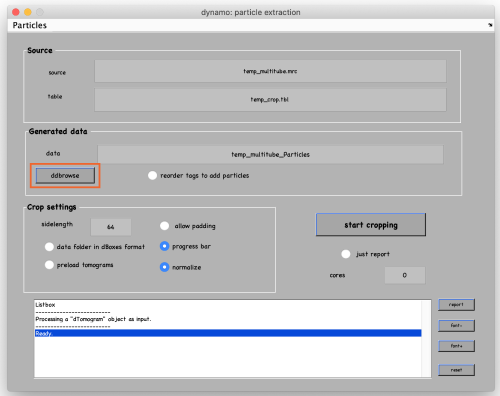
To see the results, click on ddbrowse (orange box):

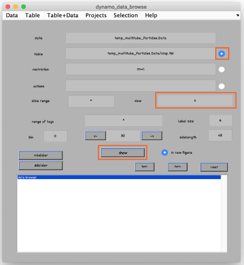
In the new window activate the table, select the axis and click on show (orange boxes):

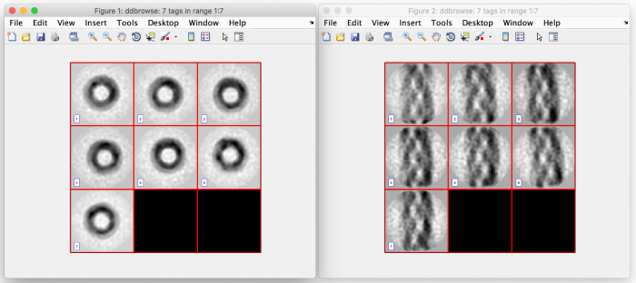
For the z and x axis you should see results similar to the following. These are 2D representations (projections) of the actually cropped 3D subtomograms: