Getting a Structure from Multiple Tomograms of HIV Capsids (walkthrough)
In this walkthrough you will get familiar with managing multiple tomograms through the Dynamo catalogue and developing strategies for alignment projects to reach a reasonable structure from a set of tomograms. You will make use of the knowledge that you acquired during the workshop and apply it to a more realistic case. It is recommended to get familiar with the advanced starters guide and the walkthrough for lattices on vesicles before starting this walkthrough. This walkthrough represents one possible solution of this exercise.
Contents
Data
We prepared a set of 6 tomograms, each containing one Immature HIV-1 virus like particle (VLP) with a layer formed by a lattice of capsid proteins. The capsid proteins have a C6 symmetry, a diameter of roughly 15nm and a molecular weight of about 150kDa. The pixelsize of the tomograms is 2.7 angstrom. You can find the tomograms in:
~/data/tutorial_VLPs
The tomograms are part of the data that was used in the publication An atomic model of HIV-1 capsid-SP1 reveals structures regulating assembly and maturation by Schur FK, Obr M, Hagen WJ, Wan W, Jakobi AJ, Kirkpatrick JM, Sachse C, Kräusslich HG and Briggs JA. (2016). The full dataset can be found on the Electron Microscopy Public Image Archive (EMPIAR) under EMPIAR-10164. The 6 tomograms were extracted from the tilt series TS_03 and TS_43.
Goal
From the data given you should be able to get a final average in which you start seeing hints of alpha helices, i.e., it should be possible to reach a resolution close to roughly 10 angstroms.
Walkthrough
Set up a catalogue
Create a new catalogue
dcm -create catVLP
and open it in the catalogue manager
dcm catVLP
You can add each volume manually to the catalogue under Catalogue -> Browse for new volume or you can make use of a volume file and add all tomograms at once under Catalogue -> Input list of tomograms -> Browse for text file (.vll file). The volume file should be created beforehand by opening a blank text file named for example VLPtomograms.vll and copy the paths of all tomograms into it:
vlp_1.mrc
vlp_2.mrc
vlp_3.mrc
vlp_4.mrc
vlp_5.mrc
vlp_6.mrc
In case you imported the tomograms using a volume file you have to click the button list volumes to refresh the tomogram list in the catalogue manager. Now you should see the 6 tomograms in the catalogue manager. Prebin the tomograms once (1x) under Catalogue -> Create binned versions -> with factor 1. You can now look at single tomograms in tomoslice by selecting a tomogram of choice in the catalogue manager and then go under View volume -> Load full prebinned Volume [if available] -> open in tomoslice. If needed, adjust the lowpass level and contrast in tomoslice to improve the depiction.
Annotate tomograms
To know where we want to later extract the subvolumes we have to first annotate the surfaces of the VLPs inside the tomograms. We do this by opening a tomogram inside tomoslice where a so called dipole Set model is defined. How to do that is described in detail in the section DipoleSet models, Corrections during picking and Corrections after picking of the walkthrough for lattices on vesicles. A new dipole set model has to be made for each tomogram. Save each model before closing tomoslice and when opening a new tomogram in tomoslice select Delete from memory if asked. In case you see markers of the previously defined dipole set inside the newly opened tomogram make sure the model pool is empty and click on reset scene before defining the new dipole set. Once you went through all tomograms click on the button list volumes inside the catalogue manager to refresh the list of tomograms. In the column model files of the tomogram list of the catalogue manager you should now see that you have one defined model per tomogram.
Define crop points
To extract subvolumes (crop particles) we need to first define the crop points on the surface of the VLPs using the previously defined models. The crop points are then stored in a table. This is all done with the following script which is an extended version of the one found in the walkthrough for lattices on vesicles. Note that we oversample the VLPs, i.e., we define enough crop points such that every protein has the chance to end up in at least one subvolume. We will take care of proteins that end up in more than subvolume in a later step. Note that this script assumes that there are exactly 6 tomograms with only one model for each tomogram. In cases where a different number of tomograms or models is used, the script has to be adapted accordingly.
% read dipole from catalogue into workspace
dcmodels catVLP -tc dipoleSet -ws o -gm 1

c=1; % counter for table
for tomo = 1:6 % loop over tomograms
    ds = o.models{tomo};                  % read models
    NDipoles = length(ds.dipoles);
    for i=1:NDipoles                      % loop over models (in our case just one per tomogram)
        v = dmodels.vesicle();            % create empty vesicle model
        v.center = ds.dipoles{i}.center;  % add center from dipole to vesicle model
        v.radius = norm( ds.dipoles{i}.north - ds.dipoles{i}.center); % add radius
        v.separation = 60;                % separation of crop points (in px)
        v.crop_distance_from_surface =0;
        v.updateCrop();                   % update vesicle model

        tv{c} = v.grepTable(); % create crop table from using vesicle model
        tv{c}(:,22) = i;       % add model number to table
        tv{c}(:,20) = tomo;    % add tomogram number to table
        c=c+1;
    end
end
In the standalone version you need to proceed as follows:
1.) Open a text file named commands.m and copy the following into the file (avoid commenting with % or #):
o=dcmodels('catVLP','tc','dipoleSet','gm',1);
c=1;
for tomo = 1:6
    ds = dread(o{tomo});
    NDipoles = length(ds.dipoles);
    for i=1:NDipoles
        v = dmodels.vesicle();
        v.center = ds.dipoles{i}.center;
        v.radius = norm( ds.dipoles{i}.north - ds.dipoles{i}.center);
        v.separation = 60;
        v.crop_distance_from_surface =0;
        v.updateCrop();
        tv{c} = v.grepTable();
        tv{c}(:,22) = i;
        tv{c}(:,20) = tomo;
        c=c+1;
        disp(sprintf('Dipole %d will provide %d crop points',i,size(v.crop_points,2)));
    end
end
dwrite(tv,'cellOfTables.mat');
2.) Execute the text file in a system shell or in the Dynamo console:
dynamo commands.m
3.) When you are back in the Dynamo console, you can load the results from the script into the workspace with
tv = dread('cellOfTables.mat');
Type whos to display the actual matlab workspace and to check if the variable tv was loaded correctly.
Write table with crop points
The tables beloning to each dipole model are stored in the cell array tv. To create one single table containing all crop points we merge all tables into one with the command
tAll = dynamo_table_merge(tv,'linear_tags',1);
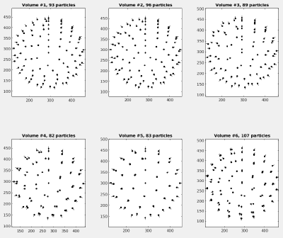
and visualize the table to see the crop points and their orientations (when visualizing actual results of an alignment project use option 'corrected_oriented_positions ' instead of the one shown here).
dtplot(tAll,'pf','oriented_positions'); axis equal
You should get something like:
Extract subvolumes
Before extracting the subvolumes (cropping particles) using the previously generated table we have to define a so called tomogram table map file which links the tomogram identification number in column 20 of the previously created table to an actual tomogram on the disk. Create a file named VLPtomograms.doc and copy the tomogram numbers and full paths of the tomograms into it:
1 vlp_1.mrc
2 vlp_2.mrc
3 vlp_3.mrc
4 vlp_4.mrc
5 vlp_5.mrc
6 vlp_6.mrc
Define a destination for the cropped particles:
targetFolder = './particlesSize128';
Now we can crop the particles with sidelength 128 pixels from the tomograms using the table previously defined.
dtcrop('VLPtomograms.doc',tAll,targetFolder,128);
The cropping on one core should not take longer than 5 minutes.
We create a plain average of all cropped particles to asses the quality of the cropped particles. First we read the table of the cropped particles:
finalTable = dread([targetFolder '/crop.tbl']);
We can also visualise the particles:
dslices(targetFolder,'projy','*','t',finalTable,'align',1,'tag',1:10:500,'labels','on');
Then we form the average
oa = daverage(targetFolder,'t',finalTable,'fc',1);
and inspect the average with
dview(oa.average)
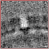
You should see a faint and noisy curvature of a thick membrane-like structure in the X and Y view.
We will use this average as a first reference (template) in the next alignment project. We therefore save the average with
dwrite(oa.average,[targetFolder '/template.em']);
Hint: When dealing with preferred orientations, randomizing the azimuth of the particles bevore averaging can help (in this tutorial this is not needed):
tRandAz = dynamo_table_randomize_azimuth(t);
First alignment project
Now we create our first alignment project through the command line in a similar way as described in detail in the walkthrough for lattices on vesicles. First we define a project name
pr = 'aliVLP';
Then we create the alignment project with the particles, template and table that we defined before. The masks are set to default.
dcp.new(pr,'d',targetFolder,'t',[targetFolder '/crop.tbl'],'template',[targetFolder '/template.em'],'masks','default','show',0);
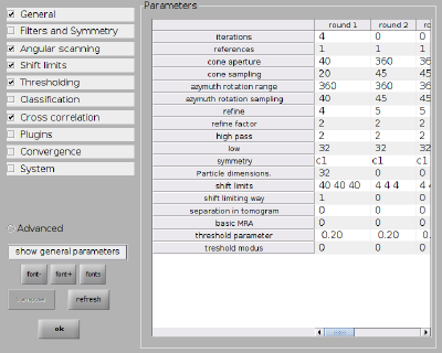
Next we set up the numerical parameters for the project and the computing environment (type dvhelp in the console for an overview of all parameters). We use 2x binned particles and a rather coarse angular search. The shift limits are very generous in order to make sure all particles have the chance to 'see' each other.
dvput(pr,'ite_r1',4);
dvput(pr,'dim_r1',32);
dvput(pr,'cr_r1',40);
dvput(pr,'cs_r1',20);
dvput(pr,'ir_r1',360);
dvput(pr,'is_r1',40);
dvput(pr,'rf_r1',4);
dvput(pr,'rff_r1',2);
dvput(pr,'lim_r1',[40,40,40]);
dvput(pr,'limm_r1',1);
dvput(pr,'dst','standalone_gpu','cores',1,'mwa',2);
Everything can of course also be set up through the alignment project GUI. The numerical parameters would correspond to:
Check, unfold and run the project through the alignment project GUI or through the command line:
dvcheck aliVLP
dvunfold aliVLP
dvrun aliVLP
On one GPU (and 2 cores for averaging) the alignment project should not take longer than half an hour. Check the status of the alignment project with
dvstatus aliVLP
You can also see the average of the last computed iteration in dmapview with the command. If needed, adjust the lowpass and contrast to improve the depiction.
dpkdev.legacy.dynamo_mapview('aliVLP:a')
Recenter and recrop
After the alignment project finished successfully we can inspect the last computed average with the same command introduced before:
dpkdev.legacy.dynamo_mapview('aliVLP:a')
The command can be extended to see the averages of all iterations including the starting reference. Once in dmapview, press the button norm to properly compare the averages.
dpkdev.legacy.dynamo_mapview('aliVLP:a:ite=0:last')
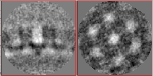
In the last average, you should already start to see a hexagonal lattice. We now want to make sure that the center of one C6 subunit of the lattice coincides with the center of the subvolume and that the subunits symmetry axis is parallel to the Z axis of the subvolume. This will allow us to later recrop the subvolumes with a smaller box size and to choose finer alignment parameters in the next alignment project. The recentering and realigning can be done in two steps. First, we subbox the particles using a new, manually defined box center and recrop the particles with a smaller boxsize. Second, we align the symmetry axis using a synthetic template. Both procedures are described in detail in the advanced starters guide in the section Aligning the axis of symmetry and Subboxing and are now applied here.
Step 1: Subboxing
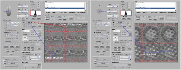
Open the last computed average in dmapview as previously described. Activate the radio buttons for the Center/North tools under Clicks. You can now click anywhere on the average and see the corresponding coordinates. Find the coordinates of the center of one subunit of the lattice. Switch between X,Y and Z view to make sure the center is correct. In our case we found the center of a subunit at [88,75,72]. For you these coordinates might be different.
Copy the found coordinates of the center of the subunit into the first vector of the command below. To compute the vector from the center of the subvolume to the center of a subunit we need to subtract the coordinates of the center of the subvolume. The center of a subvolume with a sidelength of 128 pixels is defined as [65,65,65].
rSubunitFromCenter = [88,75,72] - [65,65,65];
This vector will now be used to shift (or recenter) all particles in the table. Read the last computed table of the alignment project
ddb aliVLP:rt -ws t
and apply the new center to the table
ts = dynamo_subboxing_table(t,rSubunitFromCenter);
The table now contains the coordinates of the recentered particles. We use this new table to recrop the particles. We first define a new target folder:
targetFolder = './particlesSize96r';
Then we recrop the new particles. Since the particles are centered now, we can also choose a smaller boxsize of 96 pixels. This will save space and speed up the following processes.
dtcrop('VLPtomograms.doc',ts,targetFolder,96);
Again we average and visualize the cropping results:
finalTable = dread([targetFolder,'/crop.tbl']);
oa = daverage(targetFolder,'t',finalTable,'fc',1);
dwrite(oa.average,[targetFolder '/template.em']);
Step 2: Align symmetry axis
We see that the new average is niceley centered (there is one subunit of the lattice in the center of the volume). However, the symmetry axis is not aligned with the Z axis (the whole average looks a bit 'tilted').
We can fix that by aligning the last computed average to a synthetic template and then apply the found transformation to the table, resulting in a new and correct orientation for all particles. First we create a synthetic template using the mask tools of Dynamo. We choose a curved membrane with a hole in the center, representing the 'hollow' central subunit of the lattice.
mr = dpktomo.examples.motiveTypes.Membrane();   % create membrane object
mr.thickness  = 22;       % choose thickness of membrane
mr.sidelength = 96;       % choose sidelength of box
mr.getMask();             % compute mask
mem  = (mr.mask)*(-1)+1;  % invert contrast
cyl = dynamo_cylinder(7,96,[48,48,48]);  % create a cylinder (this will be the 'hole')
templateSum = mem+cyl;    % sum the two masks
template = templateSum;
template(template>0) = 1; % binarize the new mask
We look at the newly created template to make sure it was computed correctly.
dview(template)
Now we align the last computed average of the previous alignment project to the newly created template. We save the computed transformation parameters in the matlab object sal.
sal = dalign(oa.average,template,'cr',30,'cs',5,'ir',0,'dim',48,'limm',1,'lim',[15,15,15]);
A quick look at the newly aligned average should show a nicely centered particle with the symmetry axis aligned to the Z axis.
dmapview(sal.aligned_particle);
The transformation parameters that have been saved in the matlab object sal can now be applied to the table
tr = dynamo_table_rigid(finalTable,sal.Tp);
We now have an up-to-date table with nicely centered and aligned particles. This new table can be used in a new, finer alignment project.
Dealing with oversampling
Before starting the new alignment project we apply one more operation on the table. Since we oversampled the VLP surfaces in the beginning we might have ended up with some proteins being in more than one subvolume. Using the following function we can exclude subvolumes that are closer than 20 pixels to each other. In case the distance between two (or more) subvolumes is below this threshold, only the volume with the highest cross correlation (resulting from the previous alignment project) is kept. Read more about how to deal with oversampling here.
trEx = dpktbl.exclusionPerVolume(tr,20);
We save the new table and use it to create a new reference, which will be used in the next alignment project.
targetFolder = './particlesSize96r';
dwrite(trEx,[targetFolder '/crop_trEx.tbl']);
oa = daverage(targetFolder,'t',trEx,'fc',1);
dwrite(oa.average,[targetFolder '/template_trEx.em']);
Second aligment project
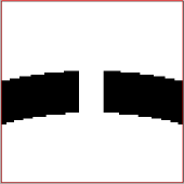
We now have particles which are centered and aligned. We dealt with the oversampling and recropped them to a smaller box size. These are good conditions to run one more alignment project with finer alignment parameters. We will narrow down the angular search, use a finer angular sampling, impose a C6 symmetry and use a tighter alignment mask. We begin by creating an alignment mask which is tighter than the previously used default one. Through the following commands we create a mask that looks like a thick curved membrane.
mr = dpktomo.examples.motiveTypes.Membrane();
mr.thickness  = 55;
mr.sidelength = 96;
mr.getMask();
mem_mask  = mr.mask;
We save the alignment mask
dwrite(mem_mask,'mem_mask_thick.em')
and inspect it in dmapview. We open first the previously created template
dmapview(oa.average)
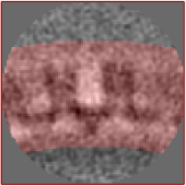
and then in the mask section we activate file, put the path of the mask in it (mem_mask_thick.em) and then click layer. You should see the mask overlaid to the average. The mask should contain all the signal of the sample. If this is not the case create a new mask with adjusted parameters.
We have now all the material to set up a new alignment project in the same way as done before. We define a new project name:
pr = 'aliVLP_fine';
We create the new alignment project with the newly cropped particles of 96 pixles sidelength, the new template and the new table. The masks are set to default for now. The new alignment mask is added in the next step.
dcp.new(pr,'d',targetFolder,'t',[targetFolder '/crop_trEx.tbl'],'template',[targetFolder '/template_trEx.em'],'masks','default','show',0);
Adding the new tight alignment mask:
dvput(pr,'file_mask','mem_mask_thick.em')
Next we set up the numerical parameters for the project. In this case we define two rounds. The first round has 2 iterations and works with 1x binned particles and a more restricted and finer angular search than the first alignment project. The second round has only 1 iteration but is using the full size particles and even finer angular search parameters. We use C6 symmetry in both rounds.
Parameters round 1:
dvput(pr,'ite_r1',2);
dvput(pr,'dim_r1',48);
dvput(pr,'cr_r1',30);
dvput(pr,'cs_r1',10);
dvput(pr,'ir_r1',30);
dvput(pr,'is_r1',10);
dvput(pr,'rf_r1',4);
dvput(pr,'rff_r1',2);
dvput(pr,'lim_r1',[15,15,15]);
dvput(pr,'limm_r1',1);
dvput(pr,'sym_r1','c6');
Parameters round 2:
dvput(pr,'ite_r2',1);
dvput(pr,'dim_r2',96);
dvput(pr,'cr_r2',12);
dvput(pr,'cs_r2',4);
dvput(pr,'ir_r2',12);
dvput(pr,'is_r2',4);
dvput(pr,'rf_r2',4);
dvput(pr,'rff_r2',2);
dvput(pr,'lim_r2',[5,5,5]);
dvput(pr,'limm_r2',2);
dvput(pr,'sym_r2','c6');
We set the computing environement:
dvput(pr,'dst','standalone_gpu','cores',1,'mwa',2);
Check, unfold and run the project:
dvcheck aliVLP_fine
dvunfold aliVLP_fine
dvrun aliVLP_fine
While the project is running, we can monitor the results in the same way as we did for the first alignment project. This project should again take no longer than half an hour on one GPU (and 2 cores for averaging). If you are under time pressure you can skip the second round. You should have already nice results after the first round.
Result
After the second alignment and without any postprocessing or elaborate refinement your final average may look similar to the one shown below. If not, it may need one more refinement round, adjustments to the mask or one more step of recentering and recropping. This representation was lowpass filtered to ~8 angstroms (or 32px in fourier space).
