Walkthrough on command line based tilt series alignment
This is the command line based version of the GUI based alignment walkthrough
Contents
Create the workflow
name = 'hivCommandLine';
folder = 'workflows';
u = dtsa(name,'--nogui','-path',folder,'fp',1);
Here, we instruct Dynamo to skip opening the GUI. We also create the workflow in a different folder.
Entering the data
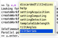
The u object contains several areas to interact with the workflow. They can be found by autocompletion using the tab key. Here, we will proceed step by step; remember that you can write all the command lines in a single .m script.
Basic data
The file of the tilt series can be defined somewhere else
file = '/~/data/b001ts001.mrc';
and then linked into the workflow:
u.enter.tiltSeries(file);
u.enter.tiltAngles(-57:3:60);
If you want to reject some of the hight tilts (or any other view that appears to have been damages,)
u.enter.discardedTiltIndices([1,40]);
Acquisition settings
Here you can enter Cs, nominal defocus, etc... We will just provide the pixel size in Angstroms:
u.enter.settingAcquisition.apix(2.7);
Computation settings
We enable the use of parallel cores
u.enter.settingComputing.parallelCPUUse(1);
This will be using mainly for gold bead detection (cc computation) and reconstruction.
To ask Dynamo to use all available physical cores, use the '*' symbol. u.enter.settingComputing.cpus('*');
Detection settings
These here are the actual design decisions when running an alignment workflow. The gold bead radius should have been measured beforehand:
u.enter.settingDetection.beadRadius(16);
u.enter.settingDetection.maskRadius(28);
u.enter.templateSidelength(64);
The bin level is mainly used to accelerate the detection procedure. Needs to be chosen in a way that a binned gold bead still can be recognisable as such, with a radius of at least 4 pixels.
u.enter.settingDetection.detectionBinningFactor(1);
Changing generic parameters
Yo can find handles to the parameters of the individuals steps through autocompletion on the area, then step items.
u.area.indexing.step.tiltGapFiller.parameterSet.residualsThreshold(8);
Running the workflow
We will skip CTF estimation and correction steps (both in the CTF area):
u.run.all('noctf',1);
If should take around five minutes to run.
Checking the results
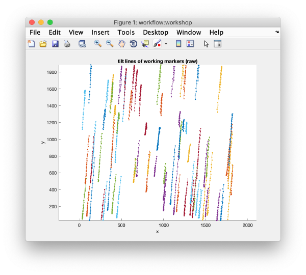
After completion, the view field allows you to check different output items for diagnose, as the tilt lines
or the reconstructions and aligned stacks themselves. You can also use the autocompletion of the info field in order to read the logs on the fit
>> u.info.fit;
------------------------------------------------------------
File with info:
  workflows/workshop2.AWF/info/fitting.doc
- - - - - - - - - - - - - - - - - - - - - - - - - - - - - -
rms:  1.39
psi: 85.10
fit modus: normal
total markers: 78
total observations: 2590
fit created at: 27-Aug-2019 18:01:40
------------------------------------------------------------
or of the markers
>> u.info.markers;
------------------------------------------------------------
Info on working markers [used during detection, indexing refinement]
  ... item saved and in memory
Item in memory:
Number of shapes          :  78
Number of frames          :  40
Number of observations    :  2590 (out of 3120)
Number of empty frames    :  2
Number of complete frames :  0
Number of complete shapes :  0

Item in disk:
Markers in disk and currently in memory contain equal coordinates

- - - - - - - - - - - - - - - - - - - - - - - - - - - - - -

Info on final markers [used from alignment step]
  ... item saved and in memory
Item in memory:
Number of shapes          :  78
Number of frames          :  40
Number of observations    :  2590 (out of 3120)
Number of empty frames    :  2
Number of complete frames :  0
Number of complete shapes :  0

Item in disk:
Markers in disk and currently in memory contain equal coordinates
------------------------------------------------------------
On the fly reconstruction of particles
In this section of the a, we show how to avoid reconstructing full tomograms of full resolution if only a set of subtomograms need to be reconstructed at high resolution. We will use the gold beads as proxies for particles of interest. We will thus locate a bunch of them in the binned tomogram, and then use their coordinates in that tomogram to directly reconstruct them in full resolution from the full resolution stack.
Grep coordinates in the binned tomogram
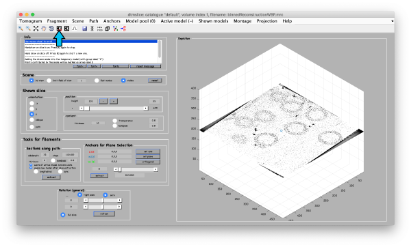
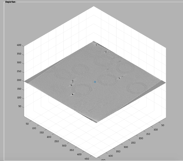
Open the binned reconstruction with dtmslice dtmslice 'workflows/hivCommandLine.AWF/reconstruction/binnedReconstructionWBP.mrc';
You will need to adjust the contrast:
Now we create a new model of general type
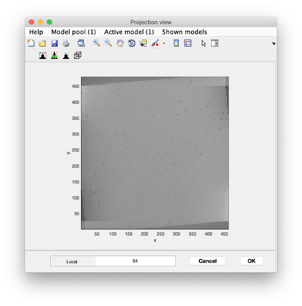
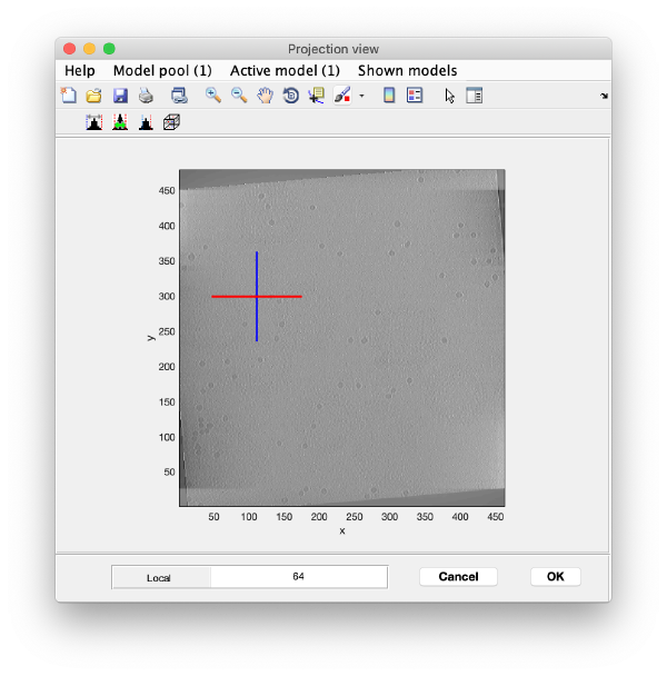
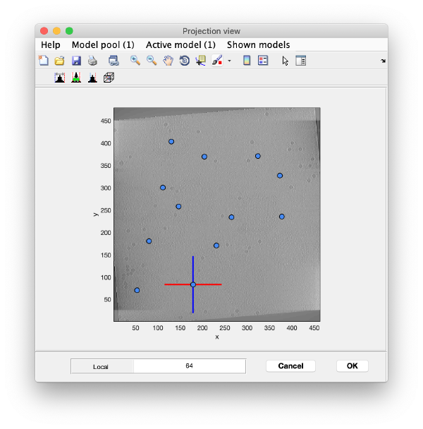
We use the projections in order to quickly find the 3d positions of a set of tomograms
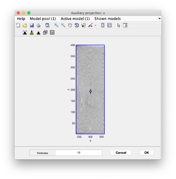
You can right click on the (x,y) position of a marker and get it depicted on its cutting xz and yz slices
Left clicking on it will provide a z coordinate to it
Keep clicking till you have a small set (no more than ten)
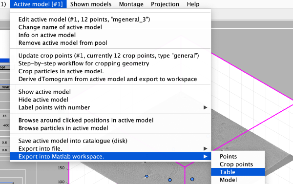
We export the coordinates of the model into the Matlab workspace already in table format, so that we will be able to use it in dtcrop on the binned tomogram.
The Matlab shell should report the variable name used to store the table.
Now we can save the table as a file: write(temp_table,'binnedGoldbeads.tbl');
Cropping the gold bead particles
We can now crop the particles using the table file
tomo = 'workflows/workshop.AWF/reconstruction/binnedReconstructionWBP.mrc';
tbl  = 'binnedGoldbeads.tbl';
targetBinnedParticles = 'binnedGoldBeads.Data';
sidelength = 32;
o = dtcrop(tomo,tbl,target,sidelength);</code>

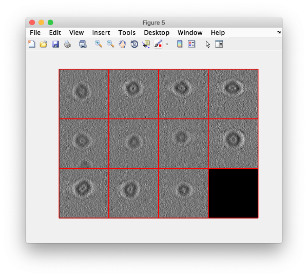
And then we visualise a projection along <tt>z</tt> of each cropped particle
 <tt>dslices(targetBinnedParticles,'proj','c');shg;</tt>

[[ File:alignCommandLine_dslicesOnBinnedGoldBeads.png |thumb|center| 600px|dslices on binned gold beads]]
Reconstruct particles on the fly
The command that reconstructs full sized particles from an aligned stack is dynama_table_trec. This is an independent function, not part of the workflow, implying that we will need to perform some format conversion.
tbl = dread('binnedGoldbeads.tbl');
We scale the table. "Bin level 2" means that each pixel in the binned tomogram is 2 times twice its size in the full resolution tomogram. This is the factor that we input into dynamo_table_rescale:
<nowiki>alignmentBinLevel = 2;
tblFull = dynamo_table_rescale(tbl,'factor',2^alignmentBinLevel); </wiki>
Now we fetch the full sized aligned stack stored inside the alignment folder:
source = 'workflows/hivCommandLine AWF/align/alignedFullStack.mrc';
We create a data folder to contain the particles to be reconstructed on the fly:
targetDirectory = 'tempCrop.Data';
Angles actually used during the reconstruction are contained in the reconstructionTiltAngles' item of the output folder. Note that they might differ from the nominal angles, as some views might have been eliminated, both explicitely by the user, of by the program not being able to align all tilts.
angles = 'workflows/hivCommandLine.AWF/align/reconstructionTiltAngles.tlt';
The (binned) coordinates were measured in a binned tomogram, whose dimensionality is requested by dynamo_table_rec. We need to provide dynamo_table_rec with visualizationTomogram = 'workflows/ hivCommandLine.AWF/reconstruction/binnedReconstructionWBP.mrc'; sizeTomogram = dynamo_read_size(visualizationTomogram); sizeTomogramFull = sizeTomogram*2^alignmentBinLevel;
The tomogram center can be shifted in order to account for a possible shift in the centre in the binned reconstruction that was used to crop the particles.
shiftTomogramCenter = [0,0,0];
We proceed now to the reconstruction.
sidelengthFullSize = 128;
dynamo_table_rec(tblFull,source,angles,targetDirectory,sidelength,....
   'applyRampFilter',1,....
   'sizeTomogram',sizeTomogramFull,....
   'shiftTomogramCenter',shiftTomogramCenter);
We can now check that the particles have been reconstructed in full size.
figure;dslices(targetDirectory,'proj','c');shg;
