Walkthrough on command line based tilt series alignment (EMBO2021)

Dynamo includes a package for automated alignment and reconstruction of tilt series. This walkthrough guides users through a series of steps on how to use it in command line based mode. The GUI based alignment walkthrough shows how to operate this procedure through the GUI. Here, we go through each command one by one.

Create the workflow

The following commands create a new alignment workflow in a separate folder. Make sure Dynamo is loaded and running (as explained in the workshop page) and type the following commands into the console. Note: The workshop setup does not allow you to copy paste commands from your desktop onto the workshop server. You need to open a browser within the workshop server and copy paste the commands from there.

name = 'hivCommandLine';
folder = 'workflows';
u = dtsa(name,'--nogui','-path',folder,'fp',1); 

Type whos to see a list of the variables that you just created with these commands.

Entering the data

The variable u is an object that contains several fields to interact with the workflow. The different fields can be found through autocompletion by pressing the enter key (see image below). In the following, these different fields will be used to pass our inputs to the workflow.

autocompletion of user object to access different fields in standalone version

Basic data

Basic data can be entered using the enter field. Here we use a binned version of the first tilt series from the EMPIAR entry 10164, depicting a set of virus like particles (VLP), which is already prepared in your working directory (see workshop page for details on how to access the directory). The file of the tilt series and the angles are passed to the workflow:

u.enter.tiltSeries('b001ts001.mrc');
u.enter.tiltAngles(-57:3:60); 

If necessary (not in this tutorial), you can use the discardedTiltIndices field to reject tilts that are of too bad quality using the following command (e.g., tilt 1 and 40):

u.enter.discardedTiltIndices([1,40]); 

Acquisition settings

Here you can enter parameters such as Cs, nominal defocus, etc. For this tutorial we just provide the pixel size in Angstroms:

u.enter.settingAcquisition.apix(2.7);

Computation settings

We enable the use of parallel cores

u.enter.settingComputing.parallelCPUUse(1); 

This will be using mainly for gold bead detection (cc computation) and reconstruction.

To use all available physical cores use:

u.enter.settingComputing.cpus('*');

Detection settings

These here are the actual design decisions when running an alignment workflow. The gold bead radius has to be known beforehand ( see GUI based alignment walkthrough on how to measure it). Binning is used internally only for quick and robust bead detection.

u.enter.settingDetection.detectionBinningFactor(1);
u.enter.settingDetection.beadRadius(16);
u.enter.settingDetection.maskRadius(28);
u.enter.templateSidelength(64);

Changing generic parameters

You can find all parameters of the individuals steps using autocompletion on the area field and then by adding step in the end. For example, the residual threshold of the tilt gap filler can be changed as follows:

u.area.indexing.step.tiltGapFiller.parameterSet.residualsThreshold(8);

Running the workflow

After setting the input parameters, the complete workflow can be run using the following command (we skip the CTF correction here). It should take about 5 minutes to run.

u.run.all('noctf',1);

Checking the results

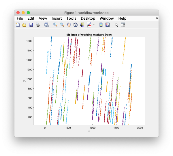
After completion, the view field allows you to check different output items for diagnose, such as the tilt lines:

u.view.tiltLines.unaligned();

view of tilt lines

or the different reconstructions

u.view.reconstruction.binnedWBP();
u.view.reconstruction.binnedSIRT();

or the aligned stacks themselves.

u.view.stack.alignedFull();

You can also use the autocompletion of the info field (as shown in the beginning) to find and display different logs:

>> u.info.fit;
------------------------------------------------------------
File with info:
  workflows/hivCommandLine.AWF/info/fitting.doc
- - - - - - - - - - - - - - - - - - - - - - - - - - - - - - 
rms:  1.41
psi: 85.20
fit modus: normal
total markers: 79
total observations: 2702
fit created at: 11-Aug-2021 10:56:24
------------------------------------------------------------

>> u.info.markers;
------------------------------------------------------------
Info on working markers [used during detection, indexing refinement]
  ... item saved and in memory
Item in memory:
Number of shapes          :  79
Number of frames          :  40
Number of observations    :  2702 (out of 3160)
Number of empty frames    :  1
Number of complete frames :  0
Number of complete shapes :  0
 
Item in disk:
Markers in disk and currently in memory contain equal coordinates
 
- - - - - - - - - - - - - - - - - - - - - - - - - - - - - - 
 
Info on final markers [used from alignment step]
  ... item saved and in memory
Item in memory:
Number of shapes          :  79
Number of frames          :  40
Number of observations    :  2702 (out of 3160)
Number of empty frames    :  1
Number of complete frames :  0
Number of complete shapes :  0
 
Item in disk:
Markers in disk and currently in memory contain equal coordinates
------------------------------------------------------------

If you are following this tutorial during a Dynamo workshop, the exercise ends here.

On the fly reconstruction of particles

In this section we show how to avoid having to reconstruct a full tomogram at full resolution for the case where only a set of subtomograms are need. For this exercise we will use the gold beads as proxies that represent any particles of interest. We will first locate a few of them in the binned tomogram, and then use those coordinates to directly reconstruct the subtomograms in full resolution and skipping the need to reconstruct the whole full sized tomogram..

Define coordinates in the binned tomogram

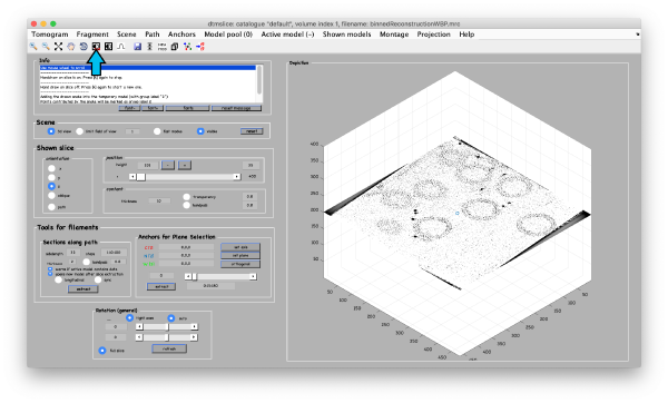
First, we open the binned reconstruction tht we created before using the visualization tool dtmslice and adjust the contrast if necessary (arrow):

dtmslice 'workflows/hivCommandLine.AWF/reconstruction/binnedReconstructionWBP.mrc';

dtmslice of binned reconstruction

dtmslice after contrast correction

To manually define the particle coordinates, we first open a new model of type general:

create a new model

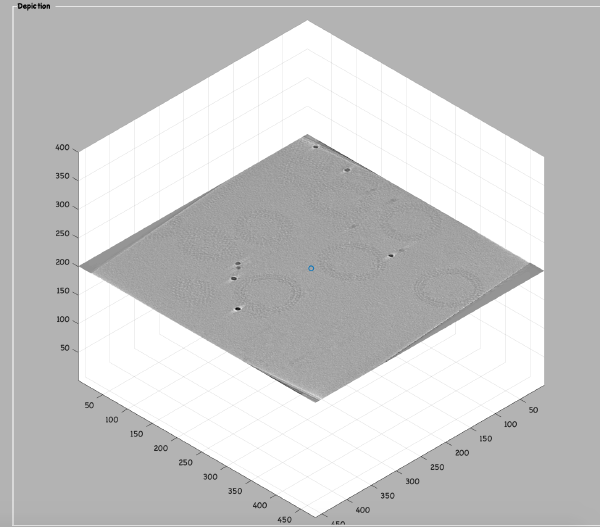
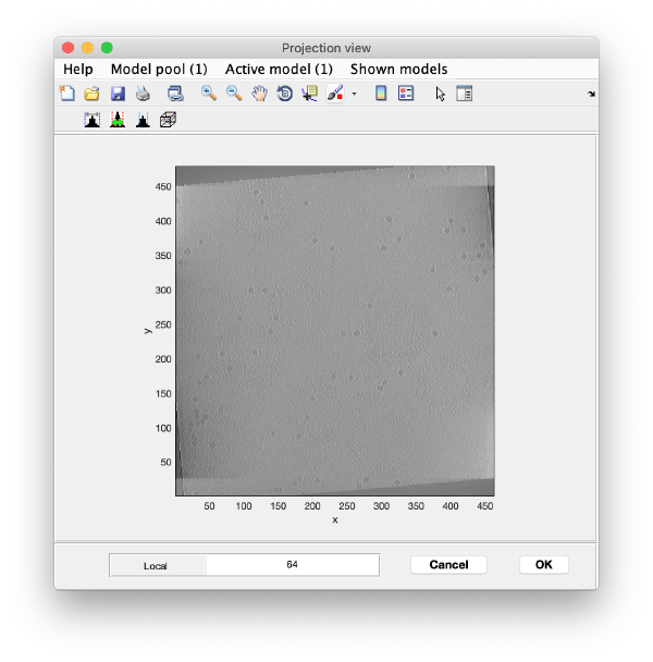
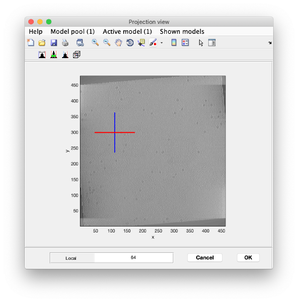
To quickly find the 3d positions of a set of particles, we use a projection of the tomogram:

show a full projection

full projection of binned reconstruction

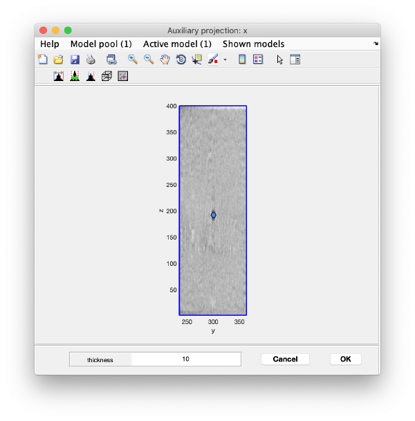
Right click on the (x,y) position of a particle opens two small windows showing the x-z and y-z planes:

right click on a point

Use the y-z depiction to left clicking on the marker. After clicking, the marker coordinates are saved in the model:

x view of clicked point

main click to fix the 3d coordinates

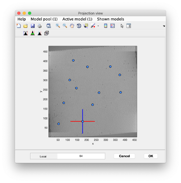
Go back to the projection view and repeat the procedure until you have a few more markers (but no more than ten in this exercise). The x-z and y-z planes will be updated automatically when clicking on new markers on the projection and do not need to be closed every time. When you are done, you can close all the plane views and also the projection view.

click around ten markers

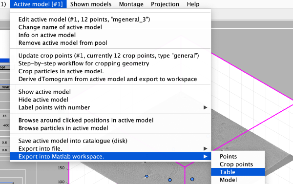
To save the coordinates we first export them into the Matlab workspace in table format:

export a table into the matlab workspace

The Matlab shell should report the variable name used to store the table:

the command line shows the variable name assigned to the created table

Now we can save the table with the coordinates as a file in the current directory (this table will be used to crop the subtomograms in the next steps):

dwrite(temp_table,'binnedGoldbeads.tbl');

Cropping the gold bead particles

We can now crop the particles using the table file that we generated before:

tomo = 'workflows/hivCommandLine.AWF/reconstruction/binnedReconstructionWBP.mrc';
tbl  = 'binnedGoldbeads.tbl';
targetBinnedParticles = 'binnedGoldBeads.Data';
sidelengthBinned = 32;
o = dtcrop(tomo,tbl, targetBinnedParticles, sidelengthBinned);

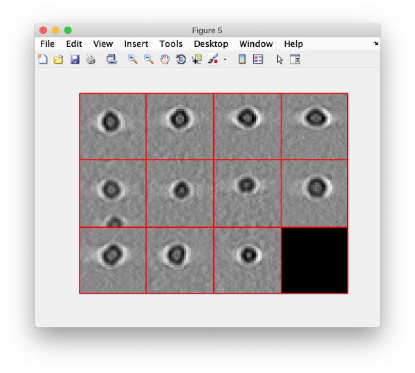
To monitor if everything worked correctly, we visualize a projection along z of each cropped particle using the command:

dslices(targetBinnedParticles,'proj','c');shg;

dslices on binned gold beads

Reconstruct particles on the fly

The command that reconstructs full sized particles from an aligned stack is dynamo_table_trec. This is an independent function, not part of the workflow, implying that we will need to perform some format conversion.

tbl     = dread('binnedGoldbeads.tbl');

We scale the table. "Bin level 2" means that each pixel in the binned tomogram is 2 times twice its size in the full resolution tomogram. This is the factor that we input into dynamo_table_rescale:

alignmentBinLevel = 2;
tblFull = dynamo_table_rescale(tbl,'factor',2^alignmentBinLevel); 

Now we fetch the full sized aligned stack stored inside the alignment folder:

source  = 'workflows/hivCommandLine.AWF/align/alignedFullStack.mrc';

We create a data folder to contain the particles to be reconstructed on the fly:

targetDirectory = 'tempCrop.Data';

Angles actually used during the reconstruction are contained in the reconstructionTiltAngles' item of the output folder. Note that they might differ from the nominal angles, as some views might have been eliminated, both explicitely by the user, of by the program not being able to align all tilts.

angles =  'workflows/hivCommandLine.AWF/align/reconstructionTiltAngles.tlt';

The (binned) coordinates were measured in a binned tomogram, whose dimensionality is requested by dynamo_table_rec. We need to provide dynamo_table_rec with

visualizationTomogram =  'workflows/hivCommandLine.AWF/reconstruction/binnedReconstructionWBP.mrc';
sizeTomogram = dynamo_read_size(visualizationTomogram);
sizeTomogramFull = sizeTomogram*2^alignmentBinLevel;

The tomogram center can be shifted in order to account for a possible shift in the centre in the binned reconstruction that was used to crop the particles.

shiftTomogramCenter = [0,0,0];

We proceed now to the reconstruction. Our sid length should be 4 times the size we used before:

sidelengthFullSize = 128;

We use the applyRampFilter option in order to explicitely estate the kind of filter that we want during the back projection.

dynamo_table_rec(tblFull,source,angles,targetDirectory, sidelengthFullSize, 'applyRampFilter',1, 'sizeTomogram',sizeTomogramFull, 'shiftTomogramCenter',shiftTomogramCenter);

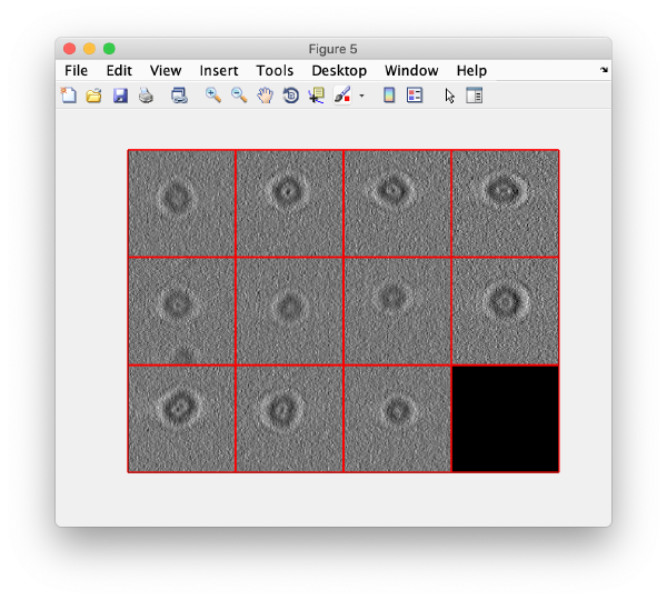
We can now check that the particles have been reconstructed in full size:

figure;dslices(targetDirectory,'proj','c');shg;

dslices on full sized gold beads