Walkthrough on membrane models

This walkthrough is a step-by-step guide that teaches how to extract subtomograms from structures with large surfaces (e.g., membranes) using the Dynamo surface models.

Data

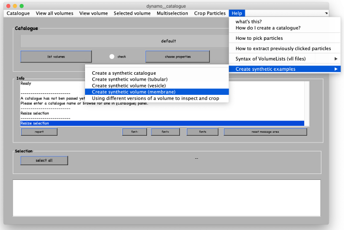
We are going to demonstrate the basic ideas and tools on a synthetic dataset. This data is already available in the catalogue manager. It can be accessed by first opening the catalogue manager using the command:

dcm

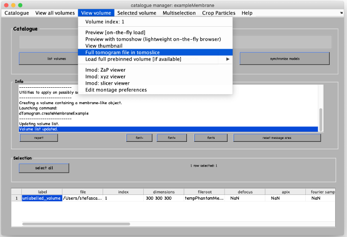
After the catalogue manager opens, we create the synthetic tomogram that includes a large surface (membrane) in the following way:

A new tomogram entry appears in the catalogue manager. Any further annotations (models) to the tomogram will be linked to this entry. Select the entry and open it:

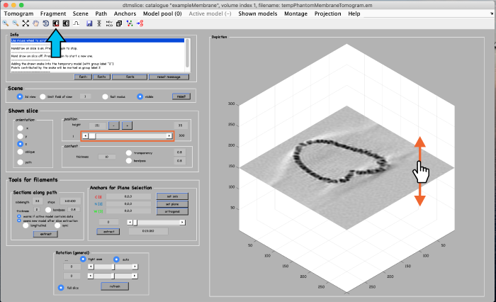
A tomogram viewer opens. You might need to adjust the contrast (blue arrow). To move through the tomogram slices, you can either use the mouse wheel, click and drag the tomogram slice up and down (orange arrows), or move the position control left and right (orange box).

Manual annotation

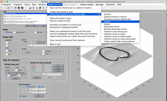
The annotation of the membrane surface is done within a so called model. We open a new model of type surface as follows:

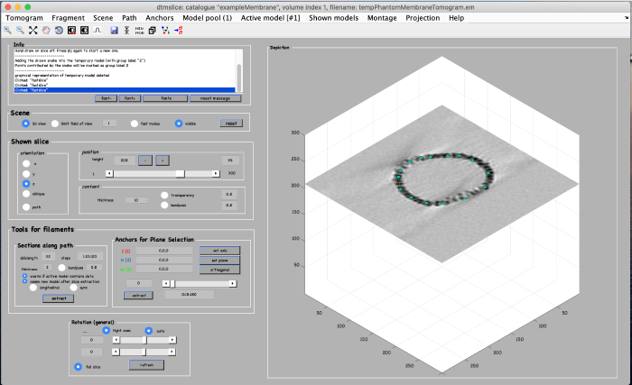
We now add manually add model points along the surface of the membrane. To do that, first move the slice up to a high z height. Then place the mouse cursor on the membrane and press the key [c] on your keyboard. This adds a new model point. Continue adding model points as shown below. Use the right-click to delete points if needed. Note: A known bug may cause the clicked points to be generated slightly displaced from the mouse cursor. Maximize the window of the tomogram viewer to get rid of this effect.

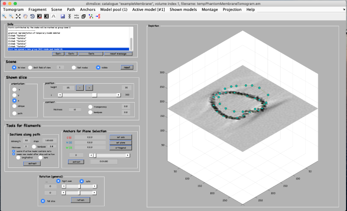
Move the slice down a bit and continue adding points on this new height as shown below:

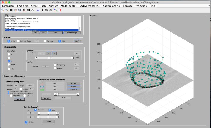
Repeat this procedure for the full structure until you get something similar to the results shown below:

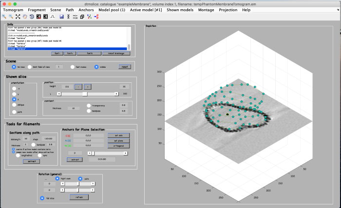
We now need to define where is the "inside" of the structure. Move the slice somewhere in the middle, place your mouse cursor in the center of the structure and press the key combination of [shift]+[c]. A point with different color should appear, as shown below:

Generate subtomogram coordinates

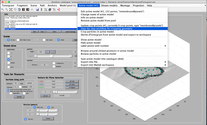
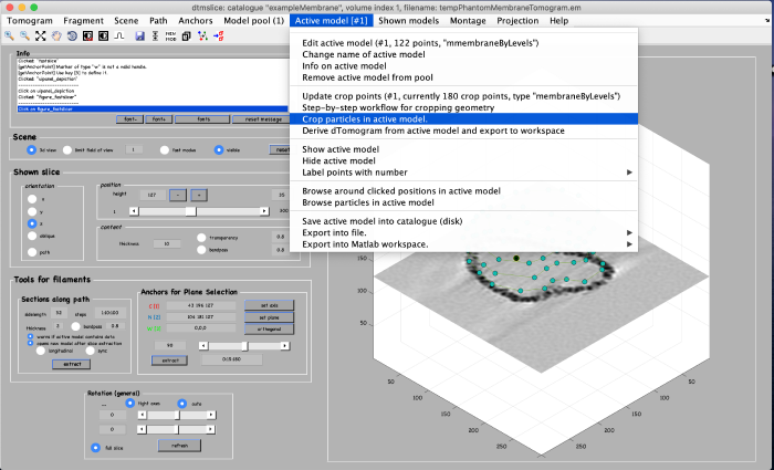
Using the clicked model we can now define the coordinates where the subvolumes will be extracted. To do that, we first processes the clicked model points using the model workflow to generate a user specific cropping geometry. Open the workflow:

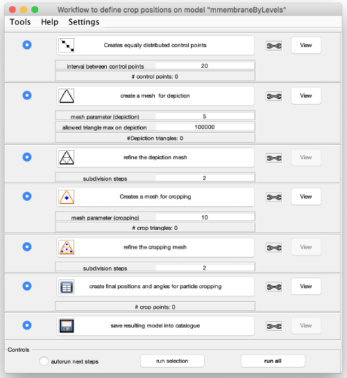
You get a new window with the model workflow. It has 7 large buttons (and corresponding input parameters below) that are executed sequentially starting from top. Click on the first button create equally distributed control points:

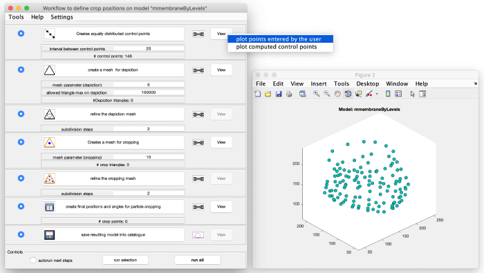
This creates equally distanced points along the points that you clicked. They will be used in the next steps to create a triangulation of the surface. Visualize your clicked points and the control points by first left-clicking on view and selecting plot points entered by user:

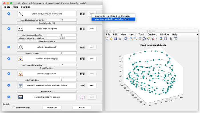
A plot with your clicked points opens. Keep it open and add the control points to the plot as shown below:

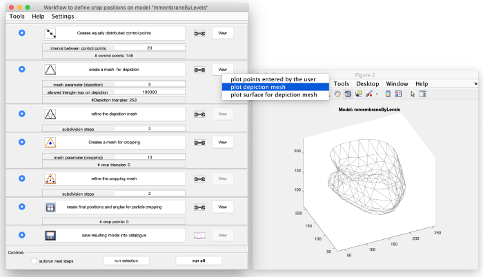
We now create two types of triangulations (or mesh). One is for depiction only and the other will be used to define the coordinates at which the subtomograms will be extracted. Both meshes are created by first generating a coarse mesh and then refining it. To create the coarse mesh for depiction first click on the create a mesh for depiction button and visualize the results:

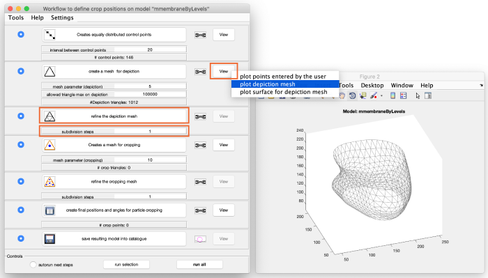
To refine the depiction mesh change the parameter subdivision steps from 2 to 1. Press the button refine the depiction mesh once and visualize the result with the view button from the previous step. You should see a finer mesh. You should also see an increase in the number for # Depiction triangles below the previous button. Clicking the refinment button again, will further refine the mesh. If you want to go back to the original mesh, simply click the button of the previous step create a mesh for depiction to overwrite the current mesh.

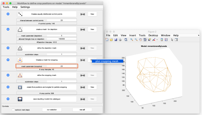
The next steps are designed to create the actual coordinates where the subtomograms will be cropped. Change the mesh parameter (cropping) from 10 to 20. This number represents the average distance between coordinates along the mesh that we just defined.

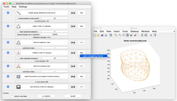
The mesh can interpreted in a way that in the center of each tile (or "triangle") one coordinate for tomogram extraction will be placed. Refine the mesh in the same way as done before by clicking once on refine the cropping mesh:

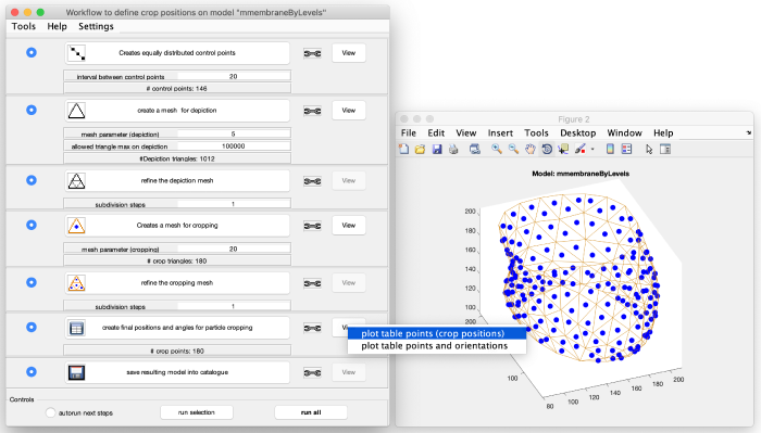
Visualize the crop positions as shown below. As you can see, each tile has one crop point in its center. In a real case you would try out different parameters until you have the coverage that fits your sample geometry. While setting those parameters, also always keep in mind the subtomogram box size that you plan to use.

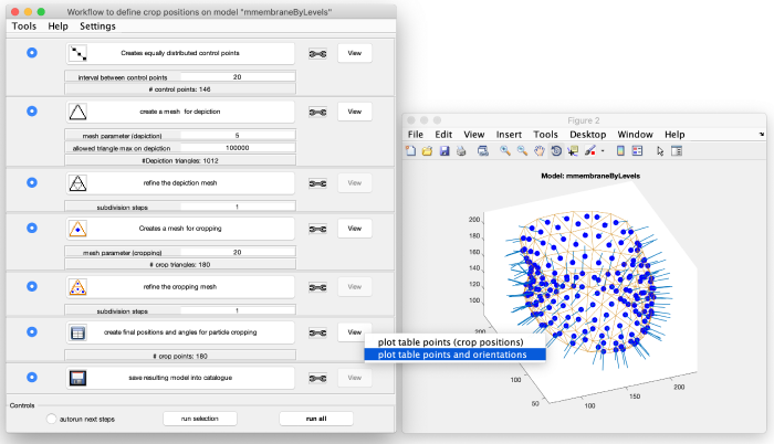
You can add the orientation of the particles to the plot as shown below. The shown orientation represents the z-axis of the particles taht will be cropped using this model. The surface model as used here imposes the z-axis to be normal to the surface:

Save the model by clicking on save resulting model into catalogue and we can move to the subtomogram extraction.

Extract subtomograms

In this final step we extract subvolumes at the coordinates defined before. First, open the partcile extraction GUI:

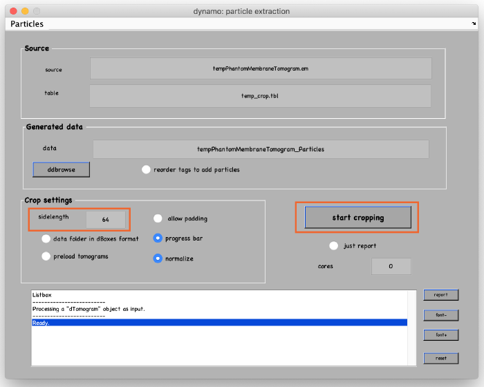
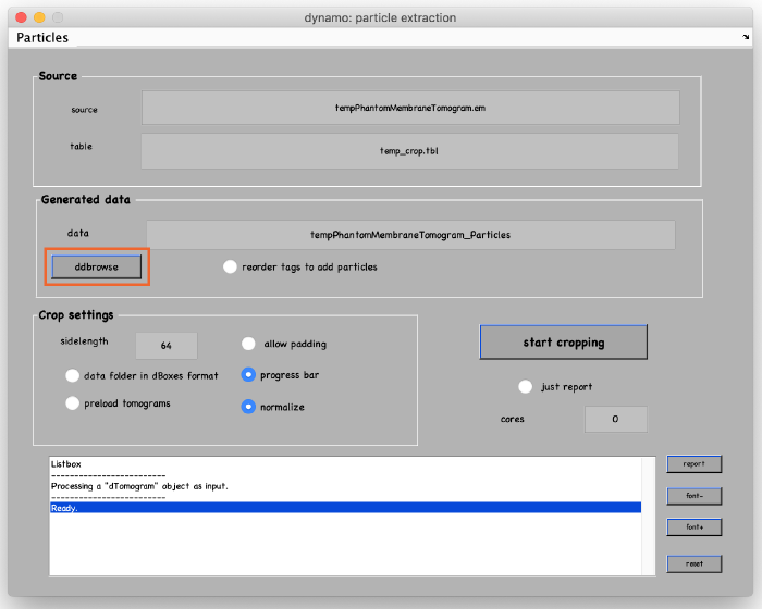
Set the sidelength to 64 and click on start cropping (orange boxes):

To see the results, click on ddbrowse (orange box):

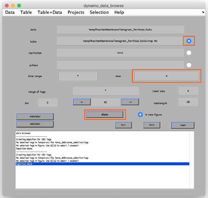
In the new window activate the table, select the x-axis and click on show (orange boxes):

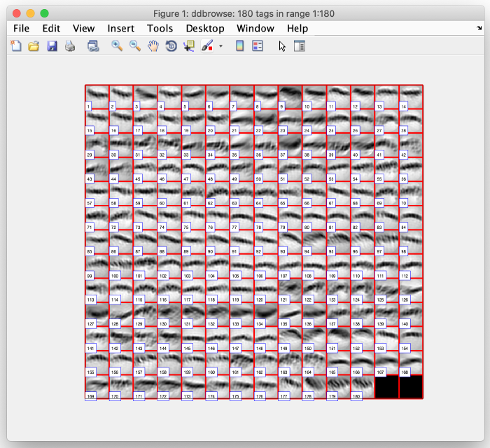
These are 2D representations (projections) of the actually cropped 3D subtomograms. Thanks to our model, the particles are already oriented having the z axis normal to the surface and the x- and y-axis are inside the membrane surface. This is why the x-view of the particles shows a cut through the membrane: