Walkthrough on localized reconstruction

ARTICLE IN CONSTRUCTION, SORRY

In this walkthrough, we use localized reconstruction to reconstruct a set of subtomograms at full pixel resolution without the requirement of creating a full reconstruction first. In this approach, we:

• create a reconstruction at low resolution
• mark the coordinates of interest in the low resolution reconstruction
• reconstruct separately the different coordinates at full resolution

For the sake of simplicity, in this walkthrough, the landmarks of interest will be simply the gold beads, which are trivially recognizable both in tomograms and in projections in the tilt series.

Example data set

The data set is an aligned tilt series. No filtering has been performed on it.

Source

The tilt series was used in the publication Cryo-EM structure of the extended type VI secretion system sheath-tube complex (J Wang et. al - Nature microbiology, 2017).

Download tilt series file

The aligned tilt series can be download from:

wget <not yet available>

This will create a file called vc17_align.ali in your current working directory. The tilt angles go from -60 to 60 in intervals of 3 degrees.

The file can be brought into memory through the command

ts = dread('vc17_align.ali');

creating the variable ts (name has been chosen arbitrarily) which contains the tilt series as a numerical matrix.

Inspecting the tilt series

The tilt series at full pixel resolution can be inspected by:

dtmshow(ts)

Prebinning during inspection

You will notice that inspecting the full series in dtmshow is bound to rather slow transitions. It is more convenient to bin the images to a smaller bin level. This can be done by switching on the binning radiobutton. Thus, the accessed slices will be binned on the fl when required.

Note that the coordinates of the axis are kept to the dimension of the unbinned tilt series.

Also, it is possible to create a prebinned version of the stack for different binning levels, so that the slice is accessed already in its prebinned dimension. This can be done after dtmshow has been initialized

or already when starting it (at the cost of an slower initialization)

dtmshow(ts,'bz',2)

Geometric conventions

In Dynamo, we call stack 3d center to a point (x_sc, y_sc,z_sc) univocally defined by a stack of micrographs:

• x_sc and z_sc and determined by the rotation axis implicitly defined by the alignment.
• y_sc is the center of the stack along direction y, defined as floor(Ny/2)+0.5; for a tilt series with Ny pixels along y.

Creation of a binned reconstruction

Binned tilt series

We bin the original tilt series:

ts2 = dpktilt.bin(ts,2)

This command applies a binning of level two to the micorgraphs in the matrix ts separately. Note that the dimensions of the new matrix are floor( [sx,sy]/2^2<2>).

Filtered tilt series

In this walkthrough, we use Weighted Backprojection as reconstruction algorithm. We apply here the simplest possible filter onto the original projections: a ramp filter.

 tsf2 = dpktomo.applyRampFilter(ts2,2)

Reconstruction

As we have binned the tiltseries, a reconstruction at the full extent of the tomogram will fit easily in memory. We need to chose a size of the output tomogram, expressed in pixels of the stack By default, the center of the reconstructed volume will be located at the stack 3d center.

obp = dpktilt.math.backproject([400,400,300],ts2,tiltAngles);

The output obp contains the reconstructed volume (as field v), and other information, including a description of the geometrical relationship between the reconstucted volume and the tilt series. We will use this information later.

CTF considerations

For simplicity, we are skipping the CTF correction step in this walkthrough, where we are only interested in the geometrical manipulations. In a real case, you would just use a version of the tilt series where each micrograph has been phase-flipped according to a defocus estimation computed on the full micrograph.

Annotation on binned reconstruction

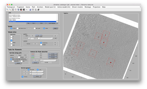
The reconstruction in bin level 2 fits in memory and can be explored easily with dtmslice

We open it creating a catalogue on the fly to contain our annotations:

dtmslice(obp.rec,'in','pr');

[[ |thumb|center|500px| Boxes-type models are the most suitable for picking in 3D]]

Annotation on 3D

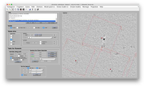
The most trivial strategy for picking particles is to use the 3D viewer. Use C to input a 3d coordinate into the model. Further controls are explained here

Select a few gold beads.

Note that you don't need to be very precise to catch the center of the gold bead.

Gold beads can be selected approximately

Annotation on projections

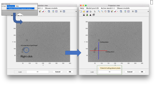
An alternative way to quickly annotate the gold beads is by concurrent projection. In this approach we launch a projection view of the full tomogram [Project > project full shown fragment alongz z].

Location of a single gold bead in the total projection viewed along z. A right click (two-finger tap on the Mac) marks the x-y position

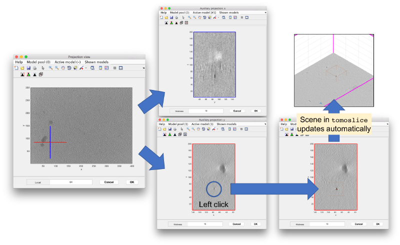
Two concurrent viewers will pop up showing cuts along x and y, i.e, YZ and XZ planes where the z coordinate can be clicked (in either of them).

A left click marks the z

The (x,y,z) point will update in the tomoslice window. Also, the windows that show the cuts long x and y will update upon new right-clicks on the z projection.

= Saving the result

On either way you click, you can save your model in the catalogue with the disk icon or under the active model menu.

Location of 3d annotations on 2d tilt series

Now we want to localize the 3d coordinates of the gold beads in the binned tilt serie. We first bring the coordinates to a memory variable that we can manipulate. 'If your dtmslice is still open, you can put the points into the workspace memory by Active Model > Export to workspace > Points, which will create in the memory a variable called temp_points with Nx3 entries. Each row are the xyz coordinates of a gold bead.

If you already closed the dtmslice session, you need to read the model that you saved into catalogue:

The points are stored as Nx3 matrix in the points property of the model.

Computation

To find the 2d coordinates of all the goldbeads at once in the micrograph corresponding to a tilt angle of -60, we would write

r2d = dpktilt.point3dInMicrograph(r3d,-60,'sc',[200.5,200.5,100.5],'ss',[sx,sy]);

Note that you need to express the geometric context of r3d.

• 'sc' stands for 'stack3dcenter'
• 'ss' stands for 'stackSize'

In other words, r3d are the coordinates of the point of interest in the reconstructed volume. You need to express how the reconstructed volume related to the original stack dpktilt.point3dInMicrograph needs this information explicitly. Alternatively, you can just use the method 'point3dInAlignedMicrograph' in the obp object, assuming it is still in memory. As this object carries the geometric information, the syntax is simpler.

 r2d = obp. point3dInAlignedMicrograph(r3d,-60);

or with the notation {} to pass position in the tilt series.

r2d = obp. point3dInAlignedMicrograph(r3d,{1});

Visualization

Basic Matlab commands

So, did it work? You can check it by just plotting the image of the micrograph

figure(); 
hi = dshow(sbin(:,:,tilt)); 

and then plotting on it the positions of the markers. hold on; h = plot(r2d(:,1),r2d(:,2),'o'); h.LineWidth=1; h.MarkerSize=10; h.Color='r';

Note that the default convention in dshow is to plot the rows of the matrix along the 'x' axis of the plot, with the origin of coordinates in the left bottom corner of the plot. The intensity of matrix entry [i,j] is represented in the pixel centered at (i-0.5,j-0.5).

Interactive GUI

The basic tool for visualizing sets of 2d markers defined on a tilt series is dmarkers. This allows to navigate at once through all the annotations on all the images. We first create a shape set for the gold beads:

ss = not yet ready 

and open the dmarkers GUI on the tilt series ts3 for this shape set:

gui = dmarkers(ts3,'ss',ss);

Remember that the gold beads had been picked loosely!

Localized reconstruction

Now we want to reconstruct locally each of the gold beads, i.e.

Reconstruction into a data folder

The command dtrec is the counterpart of dtcrop for tilt series. It loops on the positions inside a table