Walkthrough on placement of averages on table positions

In this walkthrough we show:

• how to create a triangulation that represents a density map,
• how to repeat it at the positions and orientations expressed by a Dynamo table (placement operation)
• how to visualize the same scene in Chimera:

1. through a single model for each copy of the density map
2. through a single mesh for the full scene

Creation of a density map

We will just use the ribosome32.em template inside your Dynamo installation.

%
% We create a tomogram with multiple copies of a ribosome template
% 

r = dread('ribosome32.em');

% just a normalization operation to 
rbright = dynamo_normalize_roi(r);

% inverts and normalizesit
% protein is thus dark on bright ground

%% creates a mask

% prepare a black (zeros) volume of the size of the template
mask = zeros(size(rbright));

% we select a threshold
threshold = - 0.1;

% and ellimiate densities below it
includedIndices = find(rbright>threshold);
mask(includedIndices) = rbright(includedIndices);

rbright = rbright.*mask;

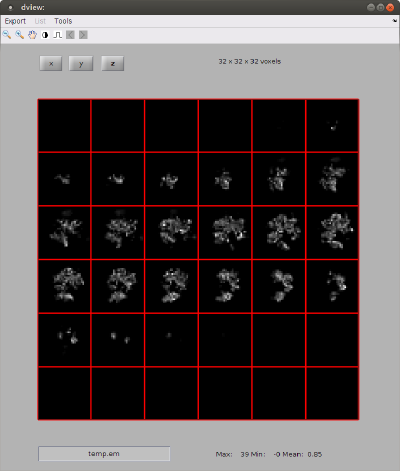
% we show the density map as a series of orthoslices
dview(rbright);

dview on the created template

Now, our task is to create a triangulation (a mesh) that represents an isosurface to be rendered later. You could just use Chimera for this, by opening the map, choosing your threshold level visually and exporting and .stl file. Alternatively, you can do it directly form the Dynamo command line with the dynamo_isosurface command.

Polishing the template triangulation

Here we show some functions in the <tt>mbgeom.triangulation</tt> package that can be used to polish the mesh.

%% 
%
% Now, we create an STL file out of the template
%

% this is a dTriRep object that covers a triangulation
% its simply a convenient wrapper around a matlab 'triangulation' object)
isolevel = 6.2;
dt = dynamo_isosurface(rbright.*mask,'isolevel',isolevel,'real_isolevel',true,'-show',false);

% we can even create a smoother surface
tSmooth = mbgeom.triangulation.smoothingSubdivision(dt.tr,'mr',1);

% the smoothing algorithm sometimes creates peaks, which can just be
% removed
tClean =  mbgeom.triangulation.removePeaks(tSmooth,'std',2);

% unconnected pieces can also be removed
tNoDust=  mbgeom.triangulation.removeDust(tClean);

% [optional]
% if we want to export a triangulation to 3D design softwares, we should 
% impose a consistent orientation for the normals of the triangles 
tFinal = mbgeom.triangulation.consistentNormals(tNoDust,'alignTo','out');

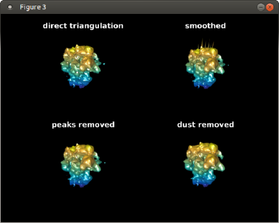
% Let's see what we just created:
figure; f = gcf; f.Name = 'construction of ribosome template';

triangulationsToPlot = {dt.tr,tSmooth,tClean,tNoDust};
titles               = {'direct triangulation','smoothed','peaks removed','dust removed'};
for i=1:4;
   ax(i) =subplot(2,2,i);
   h(i) = trisurf(triangulationsToPlot{i});
   axis('equal');
   h(i).LineStyle = 'none';
   shading(ax(i), 'interp');
   lightangle(-45,30);
   axis(ax(i),'off');
   ht(i) = title(ax(i),titles{i});
   ht(i).Color = 'w';
   mbgraph.cursors.setMouse3d(ax(i));
end

f.Color = 'k';

dview on the created template

Repeating the density map along table positions

We create first a table with random positions:

%
% table random locations for the template 
%

Nribosomes = 20;
lx = 300;
ly = 300;
lz = 400;
tb = dynamo_table_random(Nribosomes,'ts',60,'lx',300,'ly',300,'lz',300);

% we elliminate table positions that are too close to each other
tb=dpktbl.exclusionPerVolume(tb,60);

% uses round coordinates for placement of maps
tb(:,24:26) = round(tb(:,24:26));

We use to place the triangulation on the different locations of the table.

Important: you need to pass the effective rotation center of the triangulation, i.e, the point about which the rotations in the table are defined. For a volume of 32 x 32 x 32, the center is 16.5*[1,1,1];

tAll = dpktbl.triangulation.place(tb,tFinal,'rc',16.5);