Example of membrane model workflow through the command line

This excerpt of Matlab code exemplifies the operations typically operated by the cropping workflow of a membrane model. Most of the code provided here is just for creation of graphics. The important commands (i.e., the ones relevant to the handling of membrane modes) are the ones listed in des.

% creates a figure
figurePoints = figure();

% we get a handle to the axis, so that we can draw obejcts on it
haxisPoints = gca; 

% just some viewing aids:
view([1,-1,1]); % choses a viewing perspective
box on;         % creates a bounding box
axis equal;     % ensures that x,y and z units have the same proportion

% just plots the user points in the current axis
m.plotPoints(haxisPoints,'hold_limits',0);

%
% Control Points
%

% The parameter than can be changed here is:
% m.control_interval

% creates control points
m.controlUpdate();


% plots the control points in the previously avaialable axis
m.plotControlPoints(haxisPoints,'hold_limits',true);
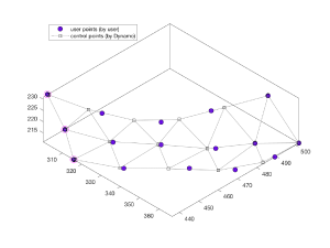
legend({'user points (by user)','control points (by Dynamo)'},'Location','northwest');
figurePoints.Name = 'From points to first triangulation';

%
% Depiction mesh
%

% we create a depiction mesh 

m.createMesh();
m.plotMesh(haxisPoints,'hold_limits',true);

This should have created this figure:

User points, control points and coarse depiction triangulation

% we refine it
m.refineMesh();

% and now plot it in a different figure;
figureMesh = figure;
haxisMesh  = gca;
view([1,-1,1]); box on; axis equal;% again some graphical support


m.plotMesh(haxisMesh,'hold_limits',false);


%%
% cropMesh
%

% provides a crop mesh parameter, which defines the mean distance between
% crop points in pixels
m.crop_mesh_parameter = 5;
m.createCropMesh();
m.plotCropMesh(haxisMesh,'hold_limits',false);
% just to put a label on the figure
figureMesh.Name='Cropping mesh on depiction mesh';

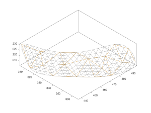
This should have created this figure:

depiction triangulation after one refinement step in black, cropping mesh in orange

%%
% final creation of table points
%
figureSketch = figure;
haxisSketch  = gca;
view([1,-1,1]); box on; axis equal;% again some graphical support

% a center (that defines laterality) should be provided
m.center = mean(m.points);
% the user can just manually pass any 3-scalar array, for instance:
% [341.8136  462.5267  220.3750]


m.updateCrop();
m.plotMesh(haxisSketch,'hold_limits',false);       % plots membrane as mesh
m.plotSurface(haxisSketch,'hold_limits',false);    % plots membrane as transparent surface
m.plotTableSketch(haxisSketch,'hold_limits',true); % plots control poins
m.plotTablePoints(haxisSketch,'hold_limits',true); %
figureSketch.Name='Cropping points and directions on depiction mesh';

%
% Output 
%

% if you want to put in back in the catalogue after the edition:
% m.saveInCatalogue();

% if you just want to get the table from this model:
% t = m.grepTable();       % it creates the t variable in the Matlab/Dynamo workspace                        
% dwrite(t,'myTable.tbl'); % writes the matrix into a file

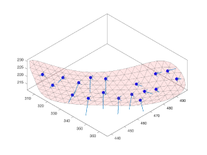
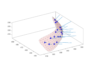
This should have created this figure:

Surface of the membrane with cropping positions and orientations

You can interactively rotate the axis of the figure for a better depiction of the orientations.

Use rotation icon to change the viewing perspective