Difference between revisions of "Walkthrough for lattices on vesicles"
| Line 53: | Line 53: | ||
=== Extracting information from the catalogue === | === Extracting information from the catalogue === | ||
| − | <nowiki>dcmodels hiv -tc dipoleSet -ws o -gm 1 | + | <nowiki>dcmodels hiv -tc dipoleSet -ws o -gm 1 |
% assumes that you only have one model file | % assumes that you only have one model file | ||
| Line 60: | Line 60: | ||
=== Create a table for each vesicle === | === Create a table for each vesicle === | ||
| − | Now we can loop on each dipole contained in the dipole set <tt>ds</tt> | + | Now we can loop on each dipole contained in the dipole set <tt>ds</tt>. |
| + | <nowiki>NDipoles = length(ds.dipoles); | ||
| + | for i=1:NDipoles; | ||
| + | v =dmodels.vesicle(); | ||
| + | |||
| + | v.center = ds.dipoles{i}.center; | ||
| + | |||
| + | % defines the radius in terms of the clicked dipole | ||
| + | v.radius = norm( ds.dipoles{i}.north - ds.dipoles{i}.center); | ||
| + | |||
| + | % create a separation distance in the vesicle | ||
| + | v.separation = 20; | ||
| + | |||
| + | % sets the cropping point 5 pixels away from the vesicle | ||
| + | % this distance in pixels is measured in the normal direction | ||
| + | v.crop_points_from_surface =2; | ||
| + | |||
| + | % creates the crop points and respective angles | ||
| + | v.updateCrop(); | ||
| + | |||
| + | % extracts a table | ||
| + | tv{i} = v.grepTable(); | ||
| + | |||
| + | % marks the table assigning in the column 22 (foreseen for arbitrary use) | ||
| + | % the number of the individual dipole | ||
| + | tv{i}(:,22) = i; | ||
| + | |||
| + | % provides information on the output | ||
| + | |||
| + | disp(sprintf('Dipole %d will provide %d crop points',i,size(v.crop_points,2))); | ||
| + | end </nowiki> | ||
=== Merging the tables === | === Merging the tables === | ||
| + | |||
| + | Each dipole with number <tt>i</tt> generated a table stored as <tt>tv{i}</tt>, i.e., the entry <tt>i</tt> inside the cell array <tt>t</tt>. We want to generate a single table. Concatenating the table matrixes will not work, as it would have several particles with the same particle tags. We thus ask ''Dynamo'' to operate the table merging by itself, and renaming the particle tags. With the order: | ||
| + | |||
| + | <tt>tAll = dynamo_table_merge(tv,'linear_tags',1);</tt> | ||
| + | |||
| + | we concatenate the tables inside the cell array <tt>tv</tt> and set the particle tags (in column 1) to be named from 1 to the maximal number of particles to be extracted from all the vesicles. You can check the result through | ||
| + | |||
| + | <tt>dtinfo(tAll);</tt> | ||
| + | |||
| + | |||
| + | or graphically through: | ||
| + | <tt>dtplot(tAll,'pf','oriented_positions');axis equal </tt> | ||
| + | |||
| + | |||
=== Create a data folder === | === Create a data folder === | ||
Revision as of 16:35, 26 July 2017
This walkthrough shows the approach to process proteins that cover spheroidal vesicles following (approximately) a structured lattice. For demonstration, we use a highly binned tomogram with several viral capsides.
Contents
Data
The data has been made available by Florian Schur . This single tomogram is part of the data set used for the paper:
Getting the data
You can download the data through the command:
dpkhelp.wiki.downloadExample('hiv');
In case this command files, please try the direct link:
wget to be filled XXX
Viewing the data
The tomogram is severely binned, so it will probably fit in memory without major problems. We can just use our typical tool to quick check a tomogram.
dtmshow v17.rec
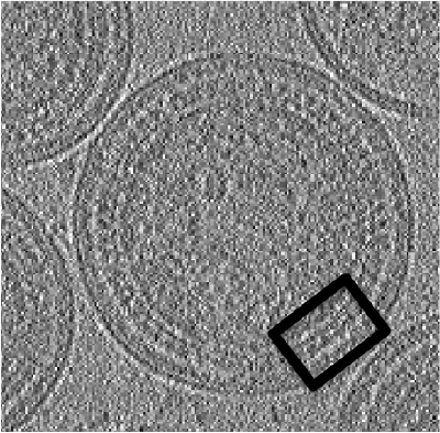
thumb|center|500px| dtmshow on the sample tomogram.
Annotation of a tomogram
We are interested in cropping the particles between the two layers of each one of the viruses.
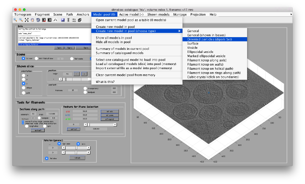
In our approach, we will first use a single model to manually input the approximate centers and radiuses of all the viruses. We will use the model type dipoleSet. This model allows to describe each annotated virus as a dipole: we will mark the (approximate) center of the virus as the center property of a dipole. The radius of the virus will be described by an annotation of the north property of the dipole.
When the model is active, we use the key c to mark the center of the current dipole, and n to mark the north. It will create a semitransparent sphere enclosing the completed dipole.
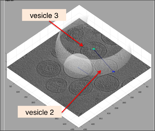
Further clicks on c or n will just move the center or the north of the same dipole. In order to click a further dipole, you need to click on enter and "open" the next dipole for clicking. If you forget to click on enter before annotating points on the next vesicle, you'll end up with situation like this:
Here, the user probably clicked on c for vesicle 2 in its real center, then clicked on n for the north point, and then moved to vesicle 3, clicking on c trying to mark the center. As a new dipole was not opened (i.e., the enter key was not pressed) when the vesicle 2 was finished, the center of vesicle 2 got misplaced. When this happens, simply press on h to hide the spheres and click the center of vesicle 2 back in its position. Then, press on enter to start the next vesicle.
When you are finished, don't forget to save the tomogram into the catalogue
Cropping the particles
We will describe a protocol to be carried from the command line, explaining each step. In short, we will visit each dipole in the model we just created, define a spherical vesicle centered on the dipole, use it to define a regular distribution of points on each vesicle, define positions pointing outwards and format everything as a table that can be used directly by Dynamo to operate an extraction and a subsequent alignment.
Extracting information from the catalogue
dcmodels hiv -tc dipoleSet -ws o -gm 1

% assumes that you only have one model file
ds = o.models{1};
Create a table for each vesicle
Now we can loop on each dipole contained in the dipole set ds.
NDipoles = length(ds.dipoles);

for i=1:NDipoles;
   v =dmodels.vesicle();

   v.center = ds.dipoles{i}.center;

   % defines the radius in terms of the clicked dipole
   v.radius = norm( ds.dipoles{i}.north - ds.dipoles{i}.center);

   % create a separation distance in the vesicle
   v.separation = 20;

   % sets the cropping point 5 pixels away from the vesicle
   % this  distance in pixels  is measured in the normal direction
   v.crop_points_from_surface =2;

   % creates the crop points and respective angles
   v.updateCrop();

   % extracts a table
   tv{i} = v.grepTable();

   % marks the table assigning in the column 22 (foreseen for arbitrary use)
   % the number of the individual dipole
   tv{i}(:,22) = i;

   % provides information on the output

   disp(sprintf('Dipole %d will provide %d crop points',i,size(v.crop_points,2)));
end
Merging the tables
Each dipole with number i generated a table stored as tv{i}, i.e., the entry i inside the cell array t. We want to generate a single table. Concatenating the table matrixes will not work, as it would have several particles with the same particle tags. We thus ask Dynamo to operate the table merging by itself, and renaming the particle tags. With the order:
tAll = dynamo_table_merge(tv,'linear_tags',1);
we concatenate the tables inside the cell array tv and set the particle tags (in column 1) to be named from 1 to the maximal number of particles to be extracted from all the vesicles. You can check the result through
dtinfo(tAll);
or graphically through:
dtplot(tAll,'pf','oriented_positions');axis equal
Create a data folder
Create an average
= Recroping the particles
help dmodels.dipoleSet.getTableFromEnclosingSpheres


