Difference between revisions of "Programmatic depiction of objects in tomograms"
| Line 57: | Line 57: | ||
will enlarge the size of the circle markers generated by the original order. | will enlarge the size of the circle markers generated by the original order. | ||
| + | Thus, a direct way to plot locations of particles coded in a [[table]] inside the scene in <tt>tomoslice</tt> would be to get the handle to the graphical axis in the currently active tomoslice session by : | ||
| + | |||
| + | <tt>axtm = dpktmslice.getAxes</tt> | ||
| + | |||
| + | setting the values of x,y,z, in terms of the information in the table: | ||
| + | <nowiki> | ||
| + | x = t(:,4)+t(:,24); | ||
| + | y = t(:,5)+t(:,25); | ||
| + | z = t(:,6)+t(:,26);</nowiki> | ||
| + | |||
| + | and the plotting the values in the graphic handle of tomoslice | ||
| + | <tt> h = plot3(x,y,z,'o','Parent','axtm')</tt>; | ||
==== Lines ==== | ==== Lines ==== | ||
Revision as of 16:26, 23 May 2017
This article describes some technique for generation of tomogram scenes.
While we call the different objects as "matlab-"XX, all the following explanations apply to the Dynamo command line, which inherits the graphic functionality of matlab.
Contents
Basic tool: graphic handles
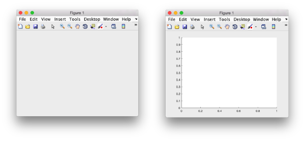
The basic objects that we will use are the matlab figure and the matlab axis. Roughly speaking, a Matlab figure is a window generated by Matlab. A Matlab axes is a system of coordinates that can be defined inside a figure, and which can contain graphical objects.
In other words, graphical objects are defined into a canvas (a Matlab axes), which is parented by a window (a Matlab figure);
Matlab figure
A matlab figure can be created just by the order;
f = figure();
Here, f is an arbitrary name,we could have called the figure any other name. Once created, this f offers a handle, i.e., a way to operate on the figure. For instance :
f.Name = 'This is my figure'
will change the name shown on the top bar of the figure.
The current figure
One can get a handle to the current figure (the last one to have been active) through the command gcf. If none is current, a new figure will be generated.
Matlab axes
A newly created figure will contain by default an axes object. The current axes can be captured through the gca command and get a handle assigned:
ax = gca
so that in the next commands we can use the variable ax to refer to the handle.
In tomography, we are normally interested in having the same scale for the x,y and z coordinates. To force an axes called ax to behave this way, we use: axes(ax,'equal');
Graphical objects
Matlab provides many primitives for depiction of 3d objects. Besides generating a graphical object, most of them will return a handle that represents the created object, and that can be used later to edit and manipulate it.
Clouds of points
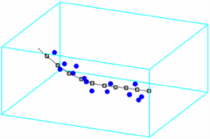
If you have three vectors x,y,z you can depict them as a set of 3d coordinates with:
h = plot3(x,y,z,'o');
In order to make explicit in which axes you want to generate the plot, you can pass the flag 'Parent', for instance:
h = plot3(x,y,z,'o','Parent','ax');
The handle h allows you to change properties in the graphics, for instance:
h.MarkerSize = 12
will enlarge the size of the circle markers generated by the original order.
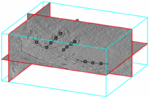
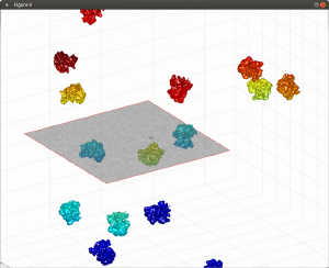
Thus, a direct way to plot locations of particles coded in a table inside the scene in tomoslice would be to get the handle to the graphical axis in the currently active tomoslice session by :
axtm = dpktmslice.getAxes
setting the values of x,y,z, in terms of the information in the table:

x = t(:,4)+t(:,24);
y = t(:,5)+t(:,25);
z = t(:,6)+t(:,26);
and the plotting the values in the graphic handle of tomoslice
h = plot3(x,y,z,'o','Parent','axtm');
Lines
Use the command line for simple lines between two points.
Tomogram slices
The class dpktomo.volume.slices.Slice is used to generate objects that can read oblique slices from inside a tomogram. The class dpktomo.volume.slices.SliceGraphic is used to generate the graphic representation of the slice.
(Examples will be posted, contact us if you need this functionality)
Models
Models have different plotting methods attached.
Standard plotting methods
The standard plotting methods are called plotXX, where XX can be Points, TablePoints
The regular syntax of a plotting method is:
object.method(axesHandle;)
Thus, if you want to use the method plotPoints to generate in a graphical axes ax a 3d depiction of the points contained inside a model called m, your syntax would be:
m.plotPoints(ax);
You can check the repertory of plot methods attached to an object through
methods(m)
Other plotting methods
You can use ezplot to get a menu for the different plot types available for an object m, i.e., enter m.ezplot() in the command line.
Tables
Placement of averages on tables
Tables and averages are the results of a subtomogram averaging experiment. As such, you frequently want to depict both of them together, by locating the computed average on the places and orientations provided by Dynamo (or any other system).
There are different techniques: you can depict the scene directly in Matlab axes, or you can use Dynamo compatibility tools to create the scene in Chimera. This can be accomplished in different formats: with the command dtchimera you create a Chimera .cmd file that generates one Chimera model for each copy of your template (on the right position and with the correct orientation). This procedure can be inconvenient if you have many models. Thus, you can also create a single triangulation that contains all the placed averages and export it into a .stl file (a format frequently used in graphics design), which Chimera can read and depict as a single model (or type Surface).
Examples cab be found on this walkthrough
