Difference between revisions of "Walkthrough on creation of 3d scenes"
| Line 38: | Line 38: | ||
Recover the last computed refined table in the data base of your project | Recover the last computed refined table in the data base of your project | ||
| − | <tt>ddb localized:rt -r t</tt> | + | <tt>ddb localized:rt -r t</tt> |
and write it to a file | and write it to a file | ||
| − | <tt>dwrite(t,'alignmentLocalRefinement.tbl') | + | <tt>dwrite(t,'alignmentLocalRefinement.tbl')</tt> |
==== Template ==== | ==== Template ==== | ||
| Line 48: | Line 48: | ||
Fetch the last computed average | Fetch the last computed average | ||
| − | <tt>ddb localizedFullAngle:rt -r a</tt> | + | <tt>ddb localizedFullAngle:rt -r a</tt> |
and write it into disk | and write it into disk | ||
| − | <tt> dwrite(t,'averagedLocalRefinement.tbl'); </tt> | + | <tt> dwrite(t,'averagedLocalRefinement.tbl'); </tt> |
==== Membrane model ==== | ==== Membrane model ==== | ||
If you [[created manually a membrane model]], it should be inside your catalogue with the name <tt>mySurface</tt> (or any other you put). You can check inside the catalogue <tt>fhv</tt>: | If you [[created manually a membrane model]], it should be inside your catalogue with the name <tt>mySurface</tt> (or any other you put). You can check inside the catalogue <tt>fhv</tt>: | ||
| − | <tt>dcmodels fhv -nc mySurf</tt> | + | <tt>dcmodels fhv -nc mySurf</tt> |
Here <tt>-nc mySurf</tt> will look for models with the string "mySurf" in the name. You should get a reply as: | Here <tt>-nc mySurf</tt> will look for models with the string "mySurf" in the name. You should get a reply as: | ||
Revision as of 17:30, 21 August 2017
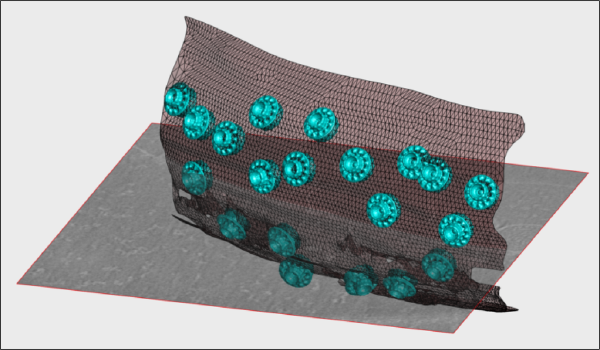
This walkthrough shows how to create graphic depictions of tomogram contents. Those include:
- Slices of tomograms.
- Proteins located in the tomogram, with the orientations provided during the alignment.
- Geometrical objects (as membranes represented by triangulations).
Contents
The data set
This walkthrough works with the data set from the advanced starters guide. The goal is to depict:
- One slice of the tomogram in 3D.
This requires a tomogram file. - The viruses placed an oriented along the directions found during a previous computed average.
This requires a template represe. - A sketch of the membrane
This requires a model object.
From the Dynamo web
The tomogram can get fetched through:
wget https://wiki.dynamo.biozentrum.unibas.ch/w/doc/data/fhv/crop.rec
in a linux shell, or through:
curl -O https://wiki.dynamo.biozentrum.unibas.ch/w/doc/data/fhv/crop.rec
under MacOS.
The table, template and membrane model can be fetched similarly with names
https://wiki.dynamo.biozentrum.unibas.ch/w/doc/data/fhv/alignmentLocalRefinement.tbl
https://wiki.dynamo.biozentrum.unibas.ch/w/doc/data/fhv/averagedLocalRefinement.em
https://wiki.dynamo.biozentrum.unibas.ch/w/doc/data/fhv/membraneModel.omd
From your previous work
Assuming you have done the tutorial on the FHV data set, you can use the elements that you have already computed. Just extract them from the best project that you completed. Do not use a subboxing project: we want to get a template for the full crown. Examples below are given assuming that your best project was named localized, substitute if not.
Table
Recover the last computed refined table in the data base of your project
ddb localized:rt -r t
and write it to a file
dwrite(t,'alignmentLocalRefinement.tbl')
Template
Fetch the last computed average
ddb localizedFullAngle:rt -r a
and write it into disk
dwrite(t,'averagedLocalRefinement.tbl');
Membrane model
If you created manually a membrane model, it should be inside your catalogue with the name mySurface (or any other you put). You can check inside the catalogue fhv:
dcmodels fhv -nc mySurf
Here -nc mySurf will look for models with the string "mySurf" in the name. You should get a reply as:
Volume 1. Matching models: 1 (total: 1) /Users/casdanie/dynamo/examples/fhvParis/fhv/tomograms/volume_1/models/mySurface.omd
So you can read the model into a new variable (arbitrarily called m)
m = drread('Users/casdanie/dynamo/examples/fhvParis/fhv/tomograms/volume_1/models/mySurface.omd');
and write it to disk
dwrite(m,'membraneModel.omd');
Depicting a slice of a tomogram
The slice object
s = dpktomo.volume.slices.Slice();
Here s is just an object that will read data from a tomogram file to be defined, along with geometrical parameters as center, eulers (orientation), l, (sidelength)...
s.source = 'crop.rec';
s.center = 'center';
Here, we set the center of the slice. We can pass a [x,y,z] triplet (like [256,200,100], or just use the code 'center' to put the center of the slice in the center of the tomogram. Now, we indicate the horizontal and vertical lengths of the slice (in pixels):
s.l = [1000,1000];
The actual extent of the slice will get cut if the l that we use is bigger than the size of the tomogram.
The orientation of the slice can be computed through a combination of euler angles [tdrort, tilt, narot], or simply with strings 'x', 'y' and 'z' for orthogonal directions. s.eulers = 'z';
Now, we actually compute the slice;
s.fetchData();
This will not create any output in the screen. fetchData will just operate the action of visiting the file crop.rec and extracting a numeric matrix that represents the gray intensities of the slice with the indicated parameters. The matrix will be stored inside the s object (as the 'data' property) and will be accessed by the depicting operations to be executed later.
The slice depictor object
We first create a figure with and empty axis f = figure; haxis = gca();hold on;
Here, f are handles that will be used later to direct the graphical output to our figure.
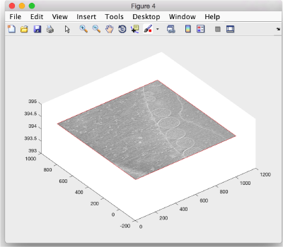
Now, we initialize a depiction object associated with the slice s sz = dpktomo.volume.slices.SliceGraphic(s); Note that no graphical output has been created yet. We first inform the object sz in which axis it is to be created.
sz.axis.h = haxis;
and then create the slice in the available axis.
sz.create();
If the figure is below other windows in your system you can rise it through
shg;
or
figure(f);
We can change the angle of view with the rotation icon or programmatically:
view([-38,60]);
Placement of templates
Here we will place copies of an FHV crown in the positions and orientations given by a table. Here, the density map representing the template needs first to be converted into an isosurface, which will be represented by a triangulation.
Creating a mask
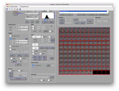
We first want to crop the available average inside a mask, to get rid of the membrane surrounding the crown. For this we first show the template inside mapview
dmapview averagedLocalRefinement.em
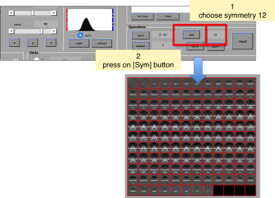
We can apply a 'c12' symmetrization on the template to get better graphical depiction.
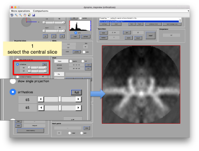
Now, we can select the area of interest by moving to the central section
[[ |thumb|center| 400px| .]]
Checking the isolevel in Chimera
You can check the appropriate isolevel using Chimera UCSF, assuming it is activated in your session.
[[ |thumb|center| 400px| .]]
[[ |thumb|center| 400px| .]]
