Difference between revisions of "Framework for estimation of membrane thickness"
| Line 6: | Line 6: | ||
<nowiki>ddb myProject:rt -d # prints in screen the last available refined table | <nowiki>ddb myProject:rt -d # prints in screen the last available refined table | ||
| − | + | ddb myProject:data -d % prints on screen the data folder linked to this project;</nowiki> | |
In any case, | In any case, | ||
| Line 64: | Line 64: | ||
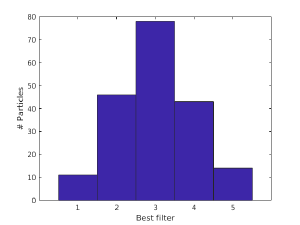
[[File:MembraneThicknessAverage.png|thumb|center|300px| Histogram of best responding membrane filters]] | [[File:MembraneThicknessAverage.png|thumb|center|300px| Histogram of best responding membrane filters]] | ||
| − | + | ||
== Creating distance filters== | == Creating distance filters== | ||
Revision as of 11:00, 9 May 2017
This framework is more useful in plastic sections. The premise is that an alignment project has been created to fix the position an orientation of a set of points of interest inside a membrane. In a later stage, we want to get an estimation on the distance between the membrane layers on each particle. This task can be performed through a multireference analysis, but it can also be approached with an analysis a posteriori as sketeched here.
Contents
Reading the particles
The easiest way to bring particles aligned by a project is through the use of the dpkdata.Reader object. First store the table and data folder of your project in variables myTable and myData. This can be easily done by browsing into the folder structure, or just by using ddb to extract items from the project. Option -d will just display the file or folder location.
ddb myProject:rt -d # prints in screen the last available refined table
ddb myProject:data -d % prints on screen the data folder linked to this project;
In any case,
r = dpkdata.Reader();
r.setSource('table', myTable,'data',myData);
you can access the particles throught the getParticle method:
p = r.getParticle(12,'align',1);
gets the particle with tag 12 as a variable p in the workspace. You can also read all the particles as a matlab cell array through
pa = r.getParticle('*','align',1);
Note that pa may have empty spaces: only the positions with an actual particle tag in the data folder will be occupied. For instance, if you don't have a particle labelled wiht 4 in your data folder, you will see it as.
>> pa

pa  =

  1×194 cell array

  Columns 1 through 5

    [96×96×96 double]    [96×96×96 double]    [96×96×96 double]    []    [96×96×96 double]

  Columns 6 through 9

    [96×96×96 double]    [96×96×96 double]    [96×96×96 double]    [96×96×96 double]
You can create a compact version of this cell array:
pac = mbg.cellCompact(pa);
>> pac

us =

  1×193 cell array

  Columns 1 through 4

    [96×96×96 double]    [96×96×96 double]    [96×96×96 double]    [96×96×96 double]

  Columns 5 through 8

   [96×96×96 double]    [96×96×96 double]    [96×96×96 double]    [96×96×96 double]
Checking the read particles
We can only measure the membrane distance on aligned particles. At this point we make certain that everything is ok by quickly adding all the particles in the cell array and checking visually the result.
myAverage = dynamo_sumarray(pac);
dview(myAverage);
Creating distance filters
We first create a set of filters that model the distance between the two layers of the membrane.
t = dpkfw.mdm.templateSeries('size',[16,16,16],'thickness',1,'distance',[3:7]);
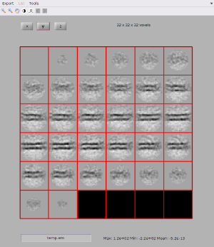
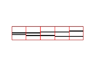
Here, t is a cell array, containing 5 volumes of 16x16x16 pixels each. Each volume contains a "model" of a membrane. You can visualize them with:
figure;dslices(t,'projy','*','dim',[1,5]);
Applying the filters onto a particle
If you have your particle in the Matlab/Dynamo workspace with name p you can type.
o = dpkfw.mdm.bestFilteringDistance(p,'templates',t);
The output structure o contains several fields with different output aspects.
>> o

o =

  output with properties:

        ok: 0
    report: {}
        cc: {[1×1 struct]  [1×1 struct]  [1×1 struct]  [1×1 struct]  [1×1 struct]}
     ccmax: [0.3385 0.3321 0.7576 0.3305 0.3393]
In particular, ccmax is telling you the response of the particle to each filter. In this case, the largest response is to the third filter in t, corresponding to an space of 5 pixels.
Loop on particles and distance histogram
Now you can put all these elements together and compute the largest response for each particle.
for i=1:length(pac)
    o = dpkfw.mdm.bestFilteringDistance(pa{i},'templates',t);
    [maxcc,myIndex] = max(o.ccmax);
    indexList(i) = myIndex(1); % in case there are two maxima
    disp(i);
end
Now, in the position i of numeric array indexList you have the index of the filter in t that responded best to the particle pa{i}. This can be depicted with the hist command in Matlab.
  figure;hist(indexList,[1:5]);
>> xlabel('Best filter');
>> ylabel('# Particles');
You'll need to convert each index to the actual number of pixels of the intermembrane space, and of course to physical units.


