Difference between revisions of "Walkthrough on PCA through the command line"
AlisterBurt (talk | contribs) m (→TSNE reduction) |
AlisterBurt (talk | contribs) |
||
| (3 intermediate revisions by the same user not shown) | |||
| Line 62: | Line 62: | ||
meaning that each block executed in parallel will preload two sets of 100 (prealigned) particles into memory, and then proceed to cross correlate all possible pairs. Ideally, you should tune your <tt>batch</tt> parameters l to have as many blocks as processing units (CPU cores or GPUs). | meaning that each block executed in parallel will preload two sets of 100 (prealigned) particles into memory, and then proceed to cross correlate all possible pairs. Ideally, you should tune your <tt>batch</tt> parameters l to have as many blocks as processing units (CPU cores or GPUs). | ||
IThis might not be possible, as it might crowd the memory of your device. Thus, in real applications you should aim at using the <tt>batch</tt> parameter to enforce a tradeoff between performance and memory usage suited to your system. | IThis might not be possible, as it might crowd the memory of your device. Thus, in real applications you should aim at using the <tt>batch</tt> parameter to enforce a tradeoff between performance and memory usage suited to your system. | ||
| + | |||
| + | If you get an error when running <tt>wb.setBatch(n);</tt> this is a bug. Try unfolding the project first (<tt>wb.unfold()</tt>), setting the batch number then unfolding again before running calculations. | ||
==== Utilities to set the batch number ==== | ==== Utilities to set the batch number ==== | ||
| Line 103: | Line 105: | ||
== Correlation matrix== | == Correlation matrix== | ||
| + | We can visualise the cross correlation matrix | ||
<tt>m=wb.getCCMatrix();</tt> | <tt>m=wb.getCCMatrix();</tt> | ||
| − | <tt>figure;dshow( | + | <tt>figure;dshow(m);h=gca();</tt> |
| + | <tt>h.YDir = 'reverse'; </tt> | ||
== Eigencomponents == | == Eigencomponents == | ||
| Line 133: | Line 137: | ||
=== Custom approach=== | === Custom approach=== | ||
You can use your own methods to visualize the eigencomponents. They can be accessed through: | You can use your own methods to visualize the eigencomponents. They can be accessed through: | ||
| − | <tt>m = | + | <tt>m = wb.getEigencomponents();</tt> |
will produce a matrix <tt>m</tt> where each column represents an eigenvector and each row a particle. Thus, to see how a particular eigencomponent distributes among the particles, you can just write: | will produce a matrix <tt>m</tt> where each column represents an eigenvector and each row a particle. Thus, to see how a particular eigencomponent distributes among the particles, you can just write: | ||
Latest revision as of 22:58, 8 February 2021
PCA computations through the command line are governed through PCA workflow objects. We describe here how to create and handle them:
Contents
Creation of a synthetic data set
dtutorial ttest128 -M 64 -N 64 -linear_tags 1 -tight 1
This generates a set of 128 particles where 64 of the, are slightly smaller than the other 64. The particle subtomogram are randomly oriented, but the alignment parameters are known.
Creation of a workflow
Input elements
The input of a PCA workflow are:
- a set of particles (called data container in this article)
- a table that expreses the alignment
- a mask that indicates the area of each alignment particle that will be taken into account during the classification procedure.
All theree have been generated by the dtutorial command.
Data
dataFolder = 'ttest128/data';
Table
tableFile = 'ttest128/real.tbl';
Mask
We create a cylindrical mask with the dimensions of the particles (40 pixels)
mask = dcylinder([20,20],40);
Syntax
We decide a name for the workflow itself, for instance
name = 'classtest128';
Now we are ready to create the workflow:
wb = dpkpca.new(name,'t',tableFile,'d',dataFolder,'m',mask);
This creates an workflow object (arbitrarily called wb) in the workspace during the current session). It also creates a folder called classtest128.PCA where results will be stored as they are produced.
Mathematical parameters
The main parameters that can be chosen in this area are:
- bandpass
wb.setBand([0,0.5,2]); % in Nyquist. % Third parameter is the smoothing factor in pixels
- symmetry
wb.setSym('c8');
- binning level (to accelerate the computations);
wb.settings.general.bin.value = 0;
Computational parameters
The main burden of the PCA computation is the creation of the cross correlation matrix.
Computing device
PCA computations can be run on GPUs of on CPUs, in both cases in parallel. In each block, two subsets of (prealigned) particles are read from disk.
To use all the available cores in your local machine, write:
wb.settings.computing.cores.value = '*';
GPU computing
By default, the ccmatrix computation will run on the CPUs. To force computation in the GPUs you need to active them first:
wb.settings.computing.useGpus.value = true;
and the specify the device numbers to use:
wb.settings.computing.gpus.value = [0:7];
In this example, you would be using 8 GPUs, marked by the systems with numbers 0 to 7.
Take into account that your system needs an independent CPU for each used GPU.
Size of parallel blocks
The size of the blocks is controlled by the parameter batch. You can tune it with:
wb.setBatch(100);
meaning that each block executed in parallel will preload two sets of 100 (prealigned) particles into memory, and then proceed to cross correlate all possible pairs. Ideally, you should tune your batch parameters l to have as many blocks as processing units (CPU cores or GPUs). IThis might not be possible, as it might crowd the memory of your device. Thus, in real applications you should aim at using the batch parameter to enforce a tradeoff between performance and memory usage suited to your system.
If you get an error when running wb.setBatch(n); this is a bug. Try unfolding the project first (wb.unfold()), setting the batch number then unfolding again before running calculations.
Utilities to set the batch number
You can get some guidance for the selection of the batch number with
wb.getBlockSize()
which will return the size of each block (in Gibabytes) for the current batch parameter. This number depends of the mask, as the block contains in memory only the part of each particle that is inside the mask.
Unfolding
Before running the workflow, it needs to be unfolded. This operation checks the mutual coherence of the different elements of the workflow, and prepares the file system for runtime.
wb.unfold();
Running
In this workflow we run the steps one by one to discuss them. In real workflows, you can use the run methods to just launch all steps sequentially.
Prealigning
wb.steps.items.prealign.compute();
Correlation matrix
All pairs of correlations are computed in blocks, as described above
wb.steps.items.ccmatrix.compute();
Eigentable
The correlation matrix is diagonalised. The eigenvectors are used to expressed as the particles as combinations of weights.
wb.steps.items.eigentable.compute();
These weights are ordered in descending order relative to their impact on the variance of the set, ideally a particle should be represented by its few components on this basis. The weights are stored in a regular Dynamo table. First eigencomponent of a particle goes into column 41.
Eigenvolumes
The eigenvectors are expressed as three=dimensional volumes.
wb.steps.items.eigenvolumes.compute();
TSNE reduction
TSNE remaps the particles into 2D maps which can be visualised and operated interactively.
wb.steps.items.tsne.compute();
Visualization
Computed elements have been stored in the workflow folder. Some of them () can be directly access through workflow tools.
Correlation matrix
We can visualise the cross correlation matrix
m=wb.getCCMatrix();
figure;dshow(m);h=gca(); h.YDir = 'reverse';
Eigencomponents
Predefined exploring tools
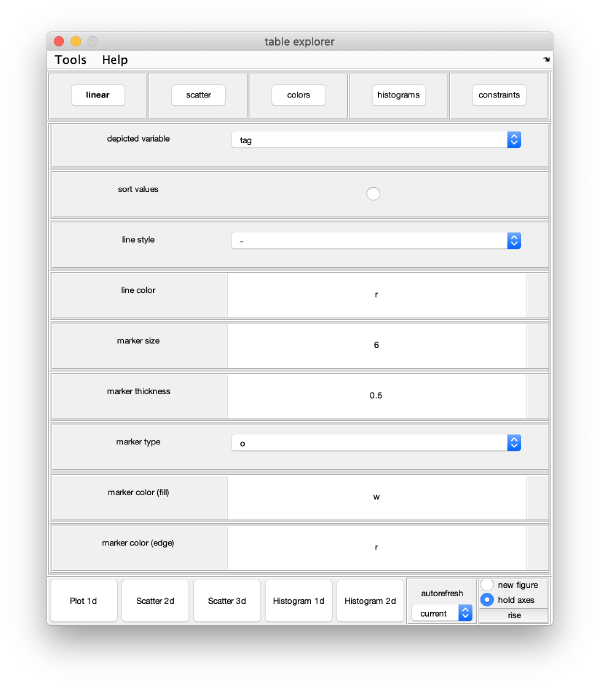
You can use a general browser for Dynamo tables:
wb.exploreGUI;
Advanced users: This is just a wrapper to the function dpktbl.gui applied on the eigentable produced by the workflow.
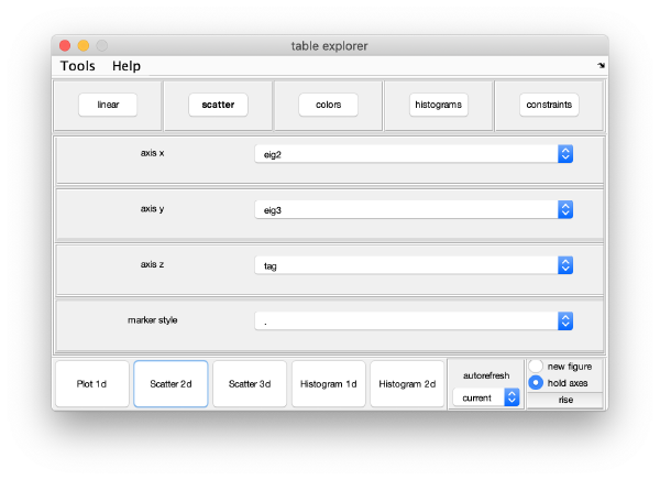
For instance, you can check how two eigencomponents relate to each other:
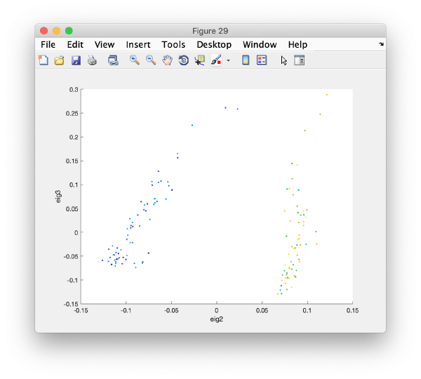
Pressing the [Scatter 2D] button will create this interactive plot
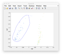
Where each point represents a different particle. Right-click on it to create a "lasso", a tool to hand-draw sets of particles.
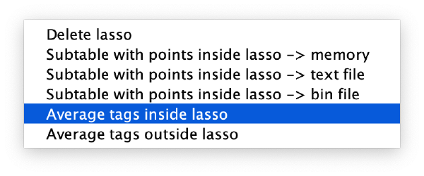
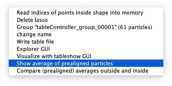
Right clicking on the "lassoed" particles give you the option of saving the information on the selected set of particles.
Custom approach
You can use your own methods to visualize the eigencomponents. They can be accessed through:
m = wb.getEigencomponents();
will produce a matrix m where each column represents an eigenvector and each row a particle. Thus, to see how a particular eigencomponent distributes among the particles, you can just write:
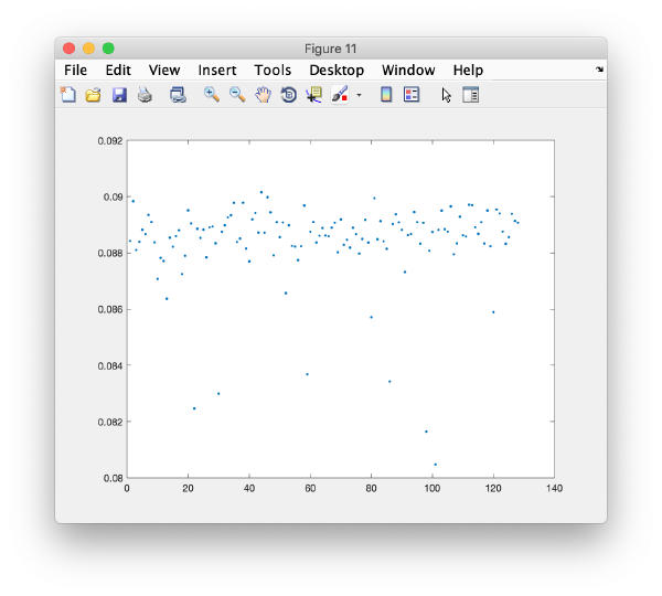
plot(m(:,i),'.');
Series of plots
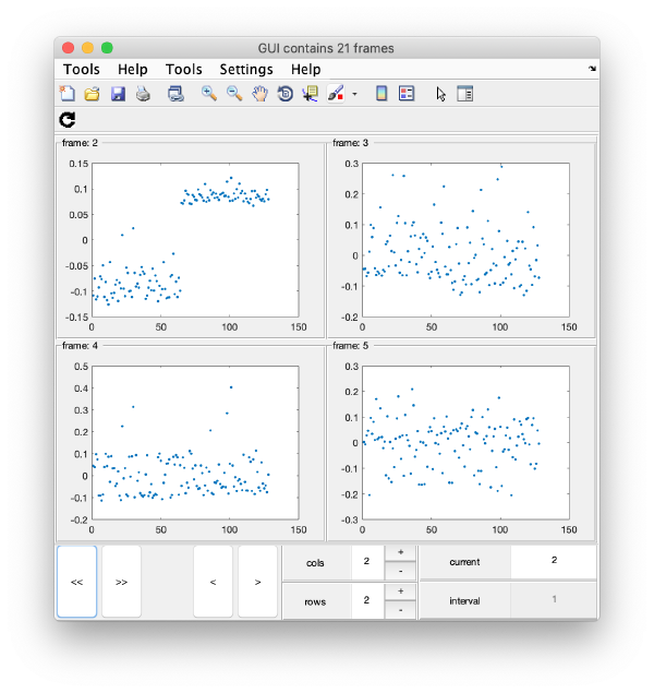
To check all the eigencomponents, it is a good idea to do some scripting. The script below uses a handy Dynamo trick to create several plots in the same figure.
 gui = mbgraph.montage();
for i=1:10
    plot(m(:,i),'.','Parent',gui.gca);
    % gui.gca captures the
      gui.step;
end
gui.first();
gui.shg();
this will produce ten plots (as i=1:10) collected in a single GUI. Each plot is called a "frame", and you can view them sequentially or in sets, just play with the layout given by the rows and columns, and use the [Refresh] icon on the top left of the GUI.
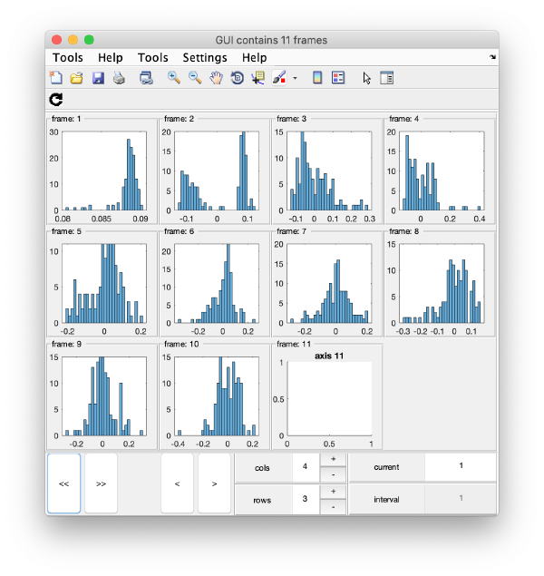
Series of histograms
Eigenvolumes
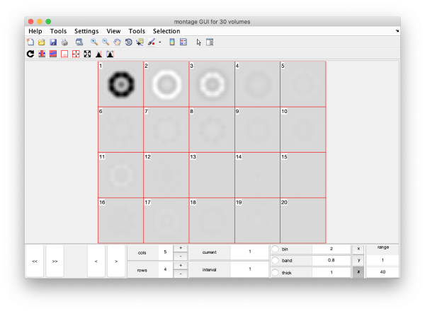
eigSet=wb.getEigenvolume(1:30);
This creates a cell array (arbitrarily called eigSet). We can visualise it through:
mbvol.groups.montage(eigSet);
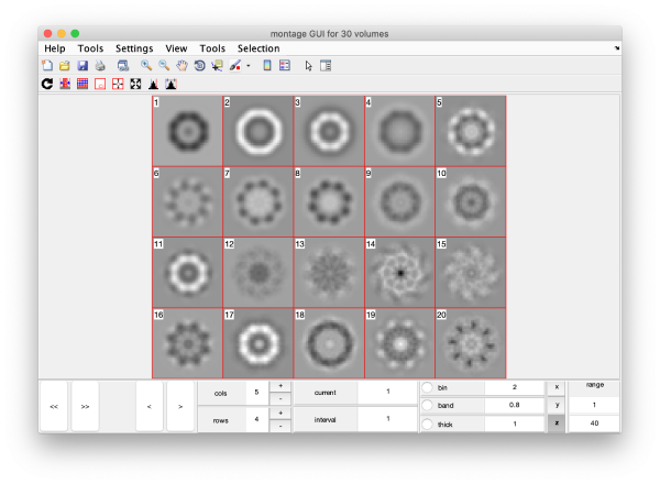
This plot is showing the true relative intensity of the eigenvolumes. In order to compare them, we can show the normalised eigenvolumes instead:
mbvol.groups.montage(dynamo_normalize_roi(eigSet));
Correlation of tilts
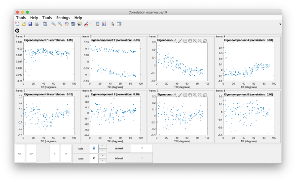
It is a good idea to check if some eigenvolumes correlate strongly with the tilt.
wb.show.correlationEigenvectorTilt(1:10)
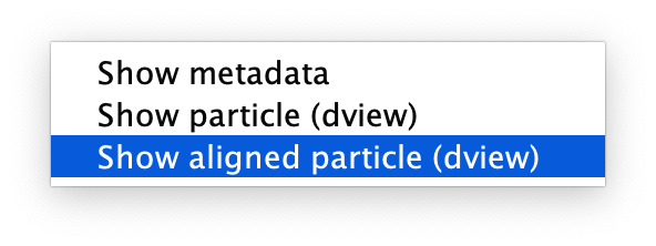
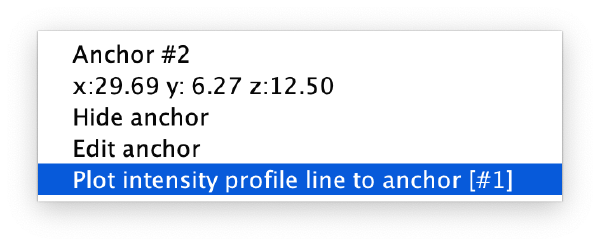
Remember that each particle is accessible through right clicking on it.
In this plot, each point represents a particle in your data set. We see that in this particular experiment, eigencomponent 3 seems to have been "corrupted by the missing wedge"
TSNE reduction
We create on the fly the TSNE reduction for eigencomponents:
wb.show.tsne([1,2,4,5]);
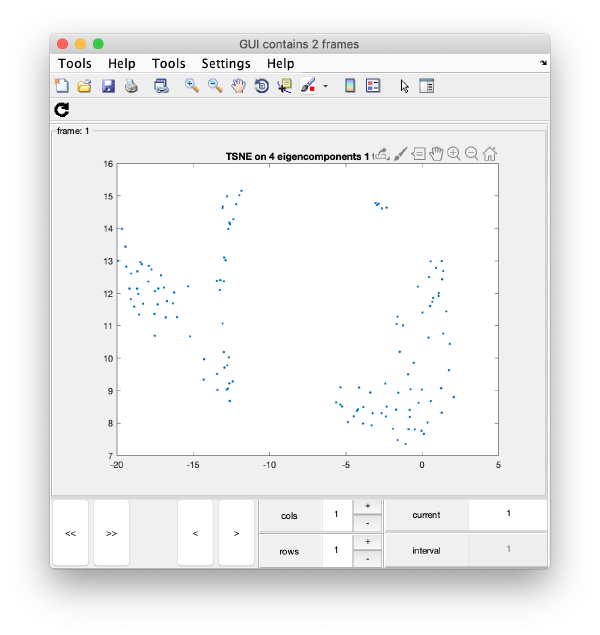
will produce the graphics:
TSNE has created a bidimensional proximity map for the 4-dimensional distribution induced by the 4 selected eigenvectors. Note that you can enter a cell array of several sets of indices. You could then navigate through different indices to check the shape of the TSNE reduction for different selections of eigenvolumes:
# wb.show.tsne({[1,2,4,5] , [1:6]});
Automated clustering
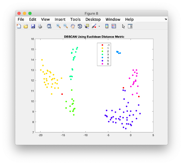
Right clicking on a plot you get an option to automatically segment it using the dbscan method
This functionality is intended to let you get a feeling of the results you would get if you would use dbscan in an algorithm.
The results are reasonable, but inferior to what human inspection would yield.
Manual clustering
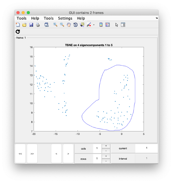
We first right click on the axis to get a lasso tool.
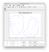
Remember that you will have a different plot (depending on the random seed used in TSNE). However, you will probably have at least a well defined cluster.
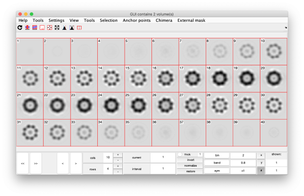
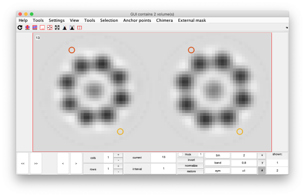
After delimiting the second subset, we can create the class averages corresponding to this manual selection.
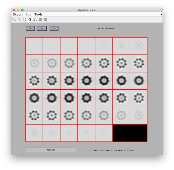
On opening, dmapview will show all slices of a single volume:
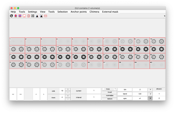
Use the "simultaneous view" icon in the toolbar to show the two volumes together.
Manipulation of PCA workflows
Reading workflows
The workflow object can be recreated by reading the workflow folder.
wb2 = dread('classtest128');
Note that we can name the workflow with an arbitrary variable name. The workflow needs to be unfolded before being used:
wb2.unfold();
This concerns not only recomputation of selected steps, but also use of graphical exploration options.
Workflow GUIs
Execution of a PCA workflow can be controlled graphically through:
wb.workflowGUI()
Overview and edition of just the workflow parameters can be accessed through:
wb.settings.editGUI
