Difference between revisions of "Walkthrough for lattices on vesicles"
| (31 intermediate revisions by 3 users not shown) | |||
| Line 9: | Line 9: | ||
You can download the data through the command: | You can download the data through the command: | ||
| − | <tt>dpkhelp.wiki.downloadExample('hiv');</tt> | + | <tt>dpkhelp.wiki.downloadExample('hiv');</tt> |
| − | In case this command | + | In case this command fails, please try the direct link in linux: |
| − | <tt> wget | + | <tt> wget https://wiki.dynamo.biozentrum.unibas.ch/w/doc/data/hiv/v17.rec</tt> |
| + | |||
| + | or the corresponding one in MacOS | ||
| + | |||
| + | <tt> curl -O https://wiki.dynamo.biozentrum.unibas.ch/w/doc/data/hiv/v17.rec</tt> | ||
=== Viewing the data === | === Viewing the data === | ||
| Line 19: | Line 23: | ||
The tomogram is severely binned, so it will probably fit in memory without major problems. We can just use our typical tool to quick check a tomogram. | The tomogram is severely binned, so it will probably fit in memory without major problems. We can just use our typical tool to quick check a tomogram. | ||
| − | <tt> dtmshow v17.rec </tt> | + | <tt> dtmshow v17.rec </tt> |
| − | [[ HivDtmshow.png |thumb|center|500px| <tt>dtmshow</tt> on the sample tomogram. ]] | + | [[ File:HivDtmshow.png |thumb|center|500px| <tt>dtmshow</tt> on the sample tomogram. ]] |
== Annotation of a tomogram == | == Annotation of a tomogram == | ||
| Line 28: | Line 32: | ||
[[ File:HivBox.png |thumb|center|400px| Structure to average]] | [[ File:HivBox.png |thumb|center|400px| Structure to average]] | ||
| + | |||
| + | We open the tomogram v17.rec with <tt>dtmslice</tt> | ||
| + | |||
| + | <tt>dtmslice v17.rec -c hiv</tt> | ||
| + | |||
| + | Here, the flag <tt>-c hiv</tt> will create a catalogue that will contain all the annotations that we perform on this volume (through the opened <tt>dtmslice</tt> session) | ||
=== DipoleSet models === | === DipoleSet models === | ||
In our approach, we will first use a single model to manually input the approximate centers and radiuses of all the viruses. We will use the model type <tt>dipoleSet</tt>. This model allows to describe each annotated virus as a ''dipole'': we will mark the (approximate) center of the virus as the <tt>center</tt> property of a dipole. The radius of the virus will be described by an annotation of the <tt>north</tt> property of the dipole. | In our approach, we will first use a single model to manually input the approximate centers and radiuses of all the viruses. We will use the model type <tt>dipoleSet</tt>. This model allows to describe each annotated virus as a ''dipole'': we will mark the (approximate) center of the virus as the <tt>center</tt> property of a dipole. The radius of the virus will be described by an annotation of the <tt>north</tt> property of the dipole. | ||
| + | |||
| + | Notice that ''Dynamo'' includes several tools for [[vesicle models]], so you might be surprised that for this particular case we go instead for this (somewhat obscurely named) ''dipoleSet'' type of model. This is just a question of convenience: the <tt>dipoleSet</tt> allows to quickly click a series of centers and radiuses and store them in a ''single'' model. That's all you need to describe vesicular geometry. Additionally, the <tt>dipoleSet</tt> includes some tools for quickly extracting particles from a ''multivesicular'' set, and it also offers a useful on-screen representation in the <tt>dtmslice</tt> tomogram browser. | ||
[[File:HivSelectModel.png|thumb|center|600px| Selecting the ''dipoleSet'' model ]] | [[File:HivSelectModel.png|thumb|center|600px| Selecting the ''dipoleSet'' model ]] | ||
| Line 49: | Line 61: | ||
=== Corrections after picking === | === Corrections after picking === | ||
| − | It is a good idea to observe your annotation from the ''x''or ''y''perspectives (for this, press on keys <tt>x</tt> or <tt>y</tt> when the cursor is on the slide). Sometimes you might identify situations like this | + | It is a good idea to observe your annotation from the ''x'' or ''y''perspectives (for this, press on keys <tt>x</tt> or <tt>y</tt> when the cursor is on the slide). Sometimes you might identify situations like this one: |
[[ File:HivWrongOnY.png|thumb|center|600px| Vesicle is too poorly picked]] | [[ File:HivWrongOnY.png|thumb|center|600px| Vesicle is too poorly picked]] | ||
| Line 67: | Line 79: | ||
We will describe a protocol to be carried from the command line, explaining each step. In short, we will visit each dipole in the model we just created, define a spherical vesicle centered on the dipole, use it to define a regular distribution of points on each vesicle, define positions pointing outwards and format everything as a [[table]] that can be used directly by ''Dynamo'' to operate an extraction and a subsequent alignment. | We will describe a protocol to be carried from the command line, explaining each step. In short, we will visit each dipole in the model we just created, define a spherical vesicle centered on the dipole, use it to define a regular distribution of points on each vesicle, define positions pointing outwards and format everything as a [[table]] that can be used directly by ''Dynamo'' to operate an extraction and a subsequent alignment. | ||
| − | === | + | === Table extraction === |
| + | |||
| + | ==== In Matlab ==== | ||
| + | |||
| + | If you are working in Matlab, you can just proceed with <tt>dcmodels</tt> to find the location of your dipole set. | ||
<nowiki>dcmodels hiv -tc dipoleSet -ws o -gm 1 | <nowiki>dcmodels hiv -tc dipoleSet -ws o -gm 1 | ||
| Line 74: | Line 90: | ||
ds = o.models{1};</nowiki> | ds = o.models{1};</nowiki> | ||
| − | === Create a table for each vesicle === | + | ===== Create a table for each vesicle ===== |
| − | Now we can loop on each dipole contained in the dipole set <tt>ds</tt>. | + | Now we can loop on each dipole contained in the dipole set <tt>ds</tt>. The next lines should be copied into a text file (using matlab command <tt>edit</tt>), and executed. |
<nowiki>NDipoles = length(ds.dipoles); | <nowiki>NDipoles = length(ds.dipoles); | ||
| Line 91: | Line 107: | ||
v.separation = 20; | v.separation = 20; | ||
| − | % sets the cropping point | + | % This parameter sets the cropping point a number of pixels away from the vesicle |
| − | % this distance in pixels is measured in the normal direction | + | % this distance in pixels is measured in the normal direction. |
| − | v. | + | % here we just use the default value. |
| + | v.crop_distance_from_surface =0; | ||
% creates the crop points and respective angles | % creates the crop points and respective angles | ||
| Line 109: | Line 126: | ||
disp(sprintf('Dipole %d will provide %d crop points',i,size(v.crop_points,2))); | disp(sprintf('Dipole %d will provide %d crop points',i,size(v.crop_points,2))); | ||
end </nowiki> | end </nowiki> | ||
| + | |||
| + | |||
| + | ==== In the standalone ==== | ||
| + | |||
| + | The standalone can execute matlab scripts, with some restrictions: the scripts need to be self contained: any traffic of variables needs to be carried through writing and reading files. There is no other possibility of transferring workspace variables between your session and the script. | ||
| + | |||
| + | ===== Creating a text file ===== | ||
| + | |||
| + | Create a text file named <tt>commands.m</tt> (arbitrary name) with any text editor available in your system. In Linux <tt>gedit</tt> is probably available. | ||
| + | |||
| + | <tt>gedit commands.m & </tt> | ||
| + | |||
| + | Now paste the text of the commands excluding comments (# simbols). | ||
| + | |||
| + | <nowiki>ds = dread(<YOUR FILE>);; | ||
| + | NDipoles = length(ds.dipoles); | ||
| + | |||
| + | for i=1:NDipoles; | ||
| + | v =dmodels.vesicle(); | ||
| + | v.center = ds.dipoles{i}.center; | ||
| + | v.radius = norm( ds.dipoles{i}.north - ds.dipoles{i}.center); | ||
| + | v.separation = 20; | ||
| + | v.crop_distance_from_surface =0; | ||
| + | v.updateCrop(); | ||
| + | tv{i} = v.grepTable(); | ||
| + | tv{i}(:,22) = i; | ||
| + | disp(sprintf('Dipole %d will provide %d crop points',i,size(v.crop_points,1))); | ||
| + | end | ||
| + | dwrite(tv,'cellOfTables.mat'); | ||
| + | </nowiki> | ||
| + | |||
| + | * Replace <tt><YOUR FILE></tt> with the actual <tt>.omd</tt> file that you created containing the dipoleSet model. | ||
| + | * Notice that we changed the variable input/output, by hardcoding the names of the files that need to be read and created. | ||
| + | |||
| + | ===== Executing the text file ===== | ||
| + | |||
| + | In a system shell or in ''Dynamo''console, type: | ||
| + | |||
| + | <tt>dynamo commands.m</tt> | ||
| + | |||
| + | ===== Getting the information back into the ''Dynamo''console ===== | ||
| + | In the ''Dynamo'' console, type. | ||
| + | <tt>tv = dread('cellOfTables.mat'); </tt> | ||
=== Merging the tables === | === Merging the tables === | ||
| Line 114: | Line 174: | ||
Each dipole with number <tt>i</tt> generated a table stored as <tt>tv{i}</tt>, i.e., the entry <tt>i</tt> inside the cell array <tt>t</tt>. We want to generate a single table. Concatenating the table matrixes will not work, as it would have several particles with the same particle tags. We thus ask ''Dynamo'' to operate the table merging by itself, and renaming the particle tags. With the order: | Each dipole with number <tt>i</tt> generated a table stored as <tt>tv{i}</tt>, i.e., the entry <tt>i</tt> inside the cell array <tt>t</tt>. We want to generate a single table. Concatenating the table matrixes will not work, as it would have several particles with the same particle tags. We thus ask ''Dynamo'' to operate the table merging by itself, and renaming the particle tags. With the order: | ||
| − | <tt>tAll = dynamo_table_merge(tv,'linear_tags',1);</tt> | + | <tt>tAll = dynamo_table_merge(tv,'linear_tags',1);</tt> |
we concatenate the tables inside the cell array <tt>tv</tt> and set the particle tags (in column 1) to be named from 1 to the maximal number of particles to be extracted from all the vesicles. You can check the result through | we concatenate the tables inside the cell array <tt>tv</tt> and set the particle tags (in column 1) to be named from 1 to the maximal number of particles to be extracted from all the vesicles. You can check the result through | ||
| − | <tt>dtinfo(tAll);</tt> | + | <tt>dtinfo(tAll);</tt> |
or graphically through: | or graphically through: | ||
| − | <tt>dtplot(tAll,'pf','oriented_positions');axis equal </tt> | + | |
| + | <tt>dtplot(tAll,'pf','oriented_positions');axis equal </tt> | ||
[[File:HivDtplotAll.png |thumb|center|600px| <tt>dtplot</tt> graphic of merged table]] | [[File:HivDtplotAll.png |thumb|center|600px| <tt>dtplot</tt> graphic of merged table]] | ||
| − | There are several programs to depict tables. In this case we may find <tt>dpktbl.plot.disks</tt> useful, as it allows to depict the particles in a table with an associated | + | There are several programs to depict tables. In this case we may find <tt>dpktbl.plot.disks</tt> useful, as it allows to depict the particles in a table with an associated extent. This is useful to check how a given sidelength in pixels covers the vesicles for a given particle distribution. |
| − | <tt>dpktbl.plots.disks(tAll,'r',10);</tt> | + | <tt>dpktbl.plots.disks(tAll,'r',10);</tt> |
[[ File:HivDisks.png|thumb|center|600px| <tt>dpktbl.plot.disks</tt> graphic of merged table]] | [[ File:HivDisks.png|thumb|center|600px| <tt>dpktbl.plot.disks</tt> graphic of merged table]] | ||
| Line 140: | Line 201: | ||
Note that that <tt>dtcrop</tt> will create a new file that contains only the particles that were actually cropped from the tomogram. Some particles were probably excluded if they were too close to the boundary of the tomogram. We can read this table file into memory. | Note that that <tt>dtcrop</tt> will create a new file that contains only the particles that were actually cropped from the tomogram. Some particles were probably excluded if they were too close to the boundary of the tomogram. We can read this table file into memory. | ||
| − | <tt>finalTable = dread([targetFolder,'/crop.tbl']);</tt> | + | <tt>finalTable = dread([targetFolder,'/crop.tbl']);</tt> |
Checking the particles can be done with the interactive browsers <tt>ddbrowse</tt> or <tt>dgallery</tt>, but for a quick check we can use the <tt>dslices</tt> command: | Checking the particles can be done with the interactive browsers <tt>ddbrowse</tt> or <tt>dgallery</tt>, but for a quick check we can use the <tt>dslices</tt> command: | ||
| − | <tt>dslices(targetFolder,'projy','*','t',finalTable,'align',1,'tag',1:10:700,'labels','on');</tt> | + | <tt>dslices(targetFolder,'projy','*','t',finalTable,'align',1,'tag',1:10:700,'labels','on');</tt> |
Here, we selected only one every ten tags to get a general idea on what is going on. The flag <tt>'projy','*'</tt> creates a projection of the aligned particles along ''y'', projecting all the slides, so that we can check that we are indeed greping the capsides. | Here, we selected only one every ten tags to get a general idea on what is going on. The flag <tt>'projy','*'</tt> creates a projection of the aligned particles along ''y'', projecting all the slides, so that we can check that we are indeed greping the capsides. | ||
| Line 156: | Line 217: | ||
We create a "coarse average" by just averaging all the particles with the orientations from the table, i.e, just the normals. | We create a "coarse average" by just averaging all the particles with the orientations from the table, i.e, just the normals. | ||
| − | <tt>oa = daverage(targetFolder,'t',finalTable,'fc',1); </tt> | + | <tt>oa = daverage(targetFolder,'t',finalTable,'fc',1); </tt> |
We can quickly check the result through: | We can quickly check the result through: | ||
| − | <tt>dview(oa)</tt> | + | <tt>dview(oa)</tt> |
[[ File:HivAverageLow.png |thumb|center|600px| <tt>view</tt> of the coarse average]] | [[ File:HivAverageLow.png |thumb|center|600px| <tt>view</tt> of the coarse average]] | ||
| − | In this case, the area of interest is probably too low in the direction 'z'. We want to lift the cropping point of the particles a little bit "downwards", that is, in the negative normal direction. | + | In this case, the area of interest is probably too low in the direction 'z': the upper half of the average is occupied by buffer. We want to lift the cropping point of the particles a little bit "downwards", that is, in the negative normal direction. |
| − | === | + | === Recropping the particles === |
Well, the protocol that we have described step by step in the previous steps can actually be completed with a single command: the method <tt>getTableFromEnclosingSpheres</tt> | Well, the protocol that we have described step by step in the previous steps can actually be completed with a single command: the method <tt>getTableFromEnclosingSpheres</tt> | ||
A complete syntax description can be found it: | A complete syntax description can be found it: | ||
| − | |||
| − | We just want to extract a data folder where the particles are better centered and have bit more of space, so that particles stamming from spheres that are poorly defined still have a chance to get driven by a posterior alignment to the center of the box. | + | <tt>help dmodels.dipoleSet.getTableFromEnclosingSpheres</tt> |
| + | |||
| + | We just want to extract a data folder where the particles are better centered and have bit more of space, so that particles stamming from spheres that are poorly defined still have a chance to get driven by a posterior alignment to the center of the box. If we initialize some variables: | ||
| + | |||
| + | <nowiki>sep = 20; % for 'separation' flag. This is the separation between particles | ||
| + | cdfs = -12; % for 'crop_distance_from_surface' flag, in pixels | ||
| + | df = 'centeredData'; % for 'dataFolder' flag. It is the data folder were the particles will be created. | ||
| + | sidelength = 64;</nowiki> | ||
| + | |||
| + | the full task can be completed in one step: | ||
| + | |||
| + | <tt>[tnew,og] = ds.getTableFromEnclosingSpheres('sep',sep,'cdfs',cdfs,'df',df,'s', sidelength,'average',1,'mw',2);</tt> | ||
| + | |||
| + | Here the <tt>mw</tt> flag just calls for 2 cores to carry the average. If you don't have a license for the Parallel Toolbox, simply don't use the flag. | ||
| + | |||
| + | Also, notice that two outputs are produced. The first one is just the table, (including also excluded particles!). The second one includes a more detailed output, including a field <tt>averageOutput</tt> that corresponds to the output of the average operation on the newly created data folder <tt>centeredData</tt>. You can view it with the normal <tt>dview</tt> command: | ||
| + | |||
| + | <tt>dview(og.averageOutput.average);</tt> | ||
| + | |||
| + | [[ File:HivAverageCentered.png |thumb|center|600px| <tt>dview</tt> on ''y'' and ''z'' of the newly computed coarse average]] | ||
| + | |||
| + | == Alignment project == | ||
| + | |||
| + | The particles can now be aligned using the table and template that we just defined. We just need to write them into files | ||
| + | |||
| + | <tt>dwrite(dread([df,'/crop.tbl']),'centered.tbl');</tt> | ||
| + | |||
| + | and the density map hidden in the output: | ||
| + | |||
| + | <tt>dwrite(og.averageOutput.average,'centered.em');</tt> | ||
| + | |||
| + | and create a [[alignment project | project]] | ||
| + | |||
| + | <tt>pr = 'pcnt'; % pr is a variable, "pcnt" is a literal string </tt> | ||
| + | |||
| + | We create an empty project pointing to the right data, template and table: | ||
| + | |||
| + | <tt>dcp.new(pr,'d',df,'t','centered.tbl','template','centered.em','masks','default','show',0);</tt> | ||
| + | |||
| + | Putting the 'show' flag to zero prevented the [[Dcp GUI | <tt>dcp</tt> GUI]] from popping up, as we want to use this walkthrough as an example of how to create and manage projects from the command line. The basic tool is <tt>dvput</tt>, which is used to change one or several project parameters. A list of the parameters and their syntax can be printed with <tt>dvhelp</tt> or consulted through the GUI <tt>dhelp</tt>. For this particular project we suggest the set below: | ||
| + | |||
| + | <nowiki>dvput(pr,'ite_r1',4); | ||
| + | dvput(pr,'dim_r1',32);</nowiki> | ||
| + | |||
| + | In the stage of finding general orientations and coarse centerings, we want to save computing time (without trading accuracy). Thus, we use the <tt>'dim_r1'</tt> parameters tune to 32. As the particle boxes have a sidelength of 64 pixels, here we are asking ''Dynamo'' to bin each particle on the fly, just one time. A neighboorhod of 2x2x2 voxels will collapse into one single voxel, with the averaged intensity. By now, we are just interested in coarsely locating the particles, so that the speed-up in the alignemnt (8x) justifies the loss of accuracy. | ||
| + | |||
| + | Next, we need angular settings reflect that we trust the normals that we have found. This will save computation time and make the alignment more robust. | ||
| + | |||
| + | <nowiki>dvput(pr,'cr_r1',40); | ||
| + | dvput(pr,'cs_r1',20); | ||
| + | dvput(pr,'ir_r1',360); | ||
| + | dvput(pr,'is_r1',40); | ||
| + | dvput(pr,'rf_r1',4); | ||
| + | dvput(pr,'rff_r1',2);</nowiki> | ||
| + | |||
| + | We let the particles shift, but not the the edges of the box: | ||
| + | |||
| + | <nowiki>dvput(pr,'lim_r1',[20,20,20]); | ||
| + | dvput(pr,'limm_r1',1);</nowiki> | ||
| + | |||
| + | Some parameters re provided to control the execution. For projects to be run in parallel under Matlab, we need the <tt>'destination'</tt> parameter tuned to value <tt>'matlab_parfor'</tt>. We also provide a value for the number of cores to be used during the alignments (parameter <tt>'cores'</tt>) and the averaging steps (parameter <tt>matlab_workers_average</tt>). | ||
| + | |||
| + | <tt>dvput(pr,'dst','matlab_parfor','cores',2,'mwa',2);</tt> | ||
| + | |||
| + | === Run project === | ||
| + | |||
| + | As we would do the GUI, we have to check, unfold and run the project: | ||
| + | |||
| + | <nowiki>dvcheck pcnt | ||
| + | dvunfold pcnt | ||
| + | dvrun pcnt</nowiki> | ||
| + | |||
| + | ==== In scripted protocols ==== | ||
| + | ''Advanced'': A note for future projects: when your own scripts to run several projects created dynamically, you can put the name of the project into a variable (as we did above) and use the <tt>( ) </tt> notation: | ||
| + | <nowiki>dvcheck(pr); | ||
| + | dvunfold(pr); | ||
| + | dvrun(pr);</nowiki> | ||
| + | When used inside a script, you probably want to use the <tt>;</tt> at the end of each line, to prevent flooding the screen with output. | ||
| + | |||
| + | === Check results === | ||
| + | |||
| + | We can check how the particles look like: | ||
| + | |||
| + | <tt>dslices('pcnt:data','projy','*','t','pcnt:rt:ite=3','align',1,'tag',1:10:700,'labels','on');</tt> | ||
| + | |||
| + | Here, <tt>'pcnt:data'</tt> is a database query. it is just a shorthand to tell ''Dynamo'' to use the data folder associated with the project <tt>pcnt</tt>. The same trick is used to extract the refined table (<tt>rt</tt>) at iteration 3. Don't worry if you don't like this notation: you can just input the actual folder and file names. | ||
| + | |||
| + | [[ File:HivDDbrowseCentered.png |thumb|center|600px| <tt> dslices </tt> of a selection of aligned particles]] | ||
| + | |||
| + | The averages can be consulted with <tt>mapview</tt>. We open the averages (<tt>a</tt> item) corresponding to iterations 0 and 4: | ||
| + | |||
| + | <tt>dpkdev.legacy.dynamo_mapview('pcnt:a:ite=[0,4]')</tt> | ||
| + | |||
| + | You can tweak the visualization to see a depiction of how the average evolved from the first template to iteration number 4. | ||
| + | |||
| + | [[ File:HivMapviewEvolution.png |thumb|center|600px| Interactive slice comparison through <tt>mapview</tt> ]] | ||
| + | |||
| + | As a tip, when you know exactly which features you want to test visually, you can use the command line order <tt>dslices</tt> to directly produce the scene of interest: | ||
| + | |||
| + | <tt>dslices pcnt:a:ite=[0,4] -projy 44 -ns 1</tt> | ||
| + | |||
| + | [[ File:HivSlicesEvolution.png|thumb|center|600px| Programatic slice comparison through <tt>dslices</tt> ]] | ||
| + | |||
| + | == Recropping the particles == | ||
| + | |||
| + | You can create a new table excluding particles that are too close to each other: | ||
| + | |||
| + | <tt>tc = dpktbl.exclusionPerVolume('pcnt:rt:ite=4',15,22);</tt> | ||
| + | |||
| + | where 15 is a distance in pixels. The third parameter denotes the column in the table that denotes particles in the same objects. In this case, we have marked each virus with a different integer in column 22 of the table, and we pass this information to <tt>dpktbl.exclusionPerVolume</tt>. | ||
Latest revision as of 13:19, 18 August 2021
This walkthrough shows the approach to process proteins that cover spheroidal vesicles following (approximately) a structured lattice. For demonstration, we use a highly binned tomogram with several viral capsides.
Contents
Data
The data has been made available by Florian Schur. This single tomogram is part of the data set used for the paper An atomic model of HIV-1 capsid-SP1 reveals structures regulating assembly and maturation by Schur FK, Obr M, Hagen WJ, Wan W, Jakobi AJ, Kirkpatrick JM, Sachse C, Kräusslich HG and Briggs JA. (2016)
Getting the data
You can download the data through the command:
dpkhelp.wiki.downloadExample('hiv');
In case this command fails, please try the direct link in linux:
wget https://wiki.dynamo.biozentrum.unibas.ch/w/doc/data/hiv/v17.rec
or the corresponding one in MacOS
curl -O https://wiki.dynamo.biozentrum.unibas.ch/w/doc/data/hiv/v17.rec
Viewing the data
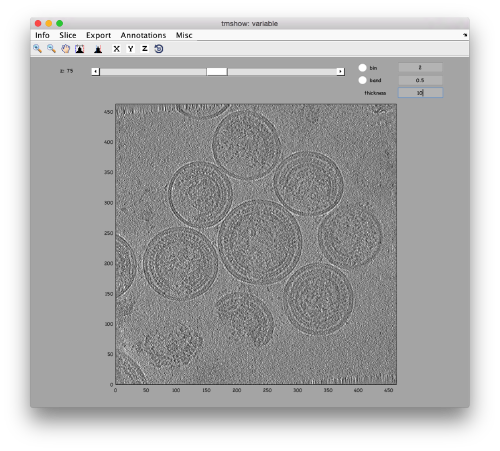
The tomogram is severely binned, so it will probably fit in memory without major problems. We can just use our typical tool to quick check a tomogram.
dtmshow v17.rec
Annotation of a tomogram
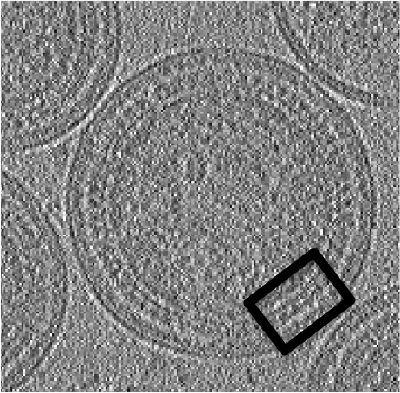
We are interested in cropping the particles between the two layers of each one of the viruses.
We open the tomogram v17.rec with dtmslice
dtmslice v17.rec -c hiv
Here, the flag -c hiv will create a catalogue that will contain all the annotations that we perform on this volume (through the opened dtmslice session)
DipoleSet models
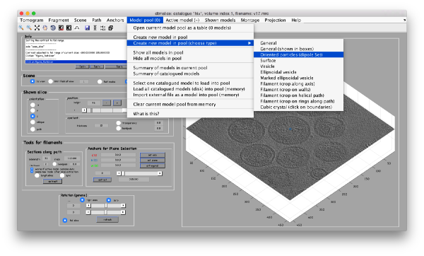
In our approach, we will first use a single model to manually input the approximate centers and radiuses of all the viruses. We will use the model type dipoleSet. This model allows to describe each annotated virus as a dipole: we will mark the (approximate) center of the virus as the center property of a dipole. The radius of the virus will be described by an annotation of the north property of the dipole.
Notice that Dynamo includes several tools for vesicle models, so you might be surprised that for this particular case we go instead for this (somewhat obscurely named) dipoleSet type of model. This is just a question of convenience: the dipoleSet allows to quickly click a series of centers and radiuses and store them in a single model. That's all you need to describe vesicular geometry. Additionally, the dipoleSet includes some tools for quickly extracting particles from a multivesicular set, and it also offers a useful on-screen representation in the dtmslice tomogram browser.
When the model is active, we use the key c to mark the center of the current dipole, and n to mark the north. It will create a semitransparent sphere enclosing the completed dipole.
Corrections during picking
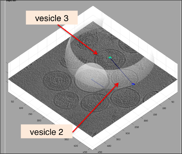
Further clicks on c or n will just move the center or the north of the same dipole. In order to click a further dipole, you need to click on enter and "open" the next dipole for clicking. If you forget to click on enter before annotating points on the next vesicle, you'll end up with situation like this:
Here, the user probably clicked on c for vesicle 2 in its real center, then clicked on n for the north point, and then moved to vesicle 3, clicking on c trying to mark the center. As a new dipole was not opened (i.e., the enter key was not pressed) when the vesicle 2 was finished, the center of vesicle 2 got misplaced. When this happens, simply press on h to hide the spheres and click the center of vesicle 2 back in its position. Then, press on enter to start the next vesicle.
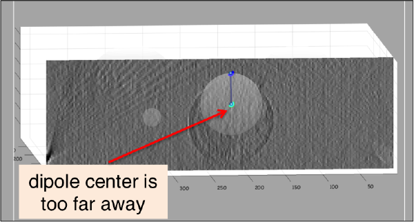
Corrections after picking
It is a good idea to observe your annotation from the x or yperspectives (for this, press on keys x or y when the cursor is on the slide). Sometimes you might identify situations like this one:
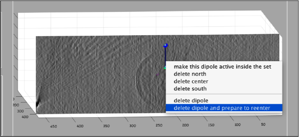
In such cases, you want to remove the dipole and click it again. The easiest way to do so is to:
- click on 'h' to hide the spheres, and
- secondary click on the wrongly created dipole (you have to click on the line itself) and select the Remove and prepare for reenter option in the menu that will popup.
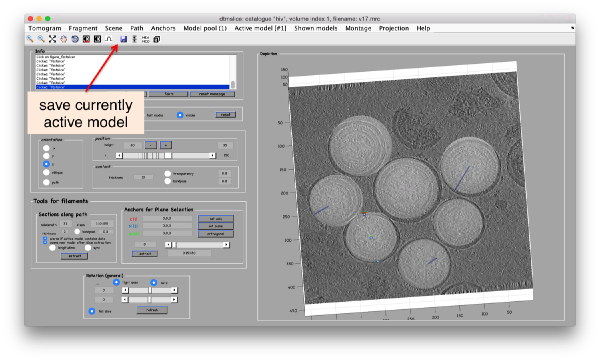
When you are finished, don't forget to save the tomogram into the catalogue, using the disk icon (or the Active Model control)
Cropping the particles
We will describe a protocol to be carried from the command line, explaining each step. In short, we will visit each dipole in the model we just created, define a spherical vesicle centered on the dipole, use it to define a regular distribution of points on each vesicle, define positions pointing outwards and format everything as a table that can be used directly by Dynamo to operate an extraction and a subsequent alignment.
Table extraction
In Matlab
If you are working in Matlab, you can just proceed with dcmodels to find the location of your dipole set.
dcmodels hiv -tc dipoleSet -ws o -gm 1

% assumes that you only have one model file
ds = o.models{1};
Create a table for each vesicle
Now we can loop on each dipole contained in the dipole set ds. The next lines should be copied into a text file (using matlab command edit), and executed.
NDipoles = length(ds.dipoles);

for i=1:NDipoles;
   v =dmodels.vesicle();

   v.center = ds.dipoles{i}.center;

   % defines the radius in terms of the clicked dipole
   v.radius = norm( ds.dipoles{i}.north - ds.dipoles{i}.center);

   % create a separation distance in the vesicle
   v.separation = 20;

   % This parameter sets the cropping point a number of pixels away from the vesicle
   % this  distance in pixels  is measured in the normal direction.
   % here we just use the default value.
   v.crop_distance_from_surface =0;

   % creates the crop points and respective angles
   v.updateCrop();

   % extracts a table
   tv{i} = v.grepTable();

   % marks the table assigning in the column 22 (foreseen for arbitrary use)
   % the number of the individual dipole
   tv{i}(:,22) = i;

   % provides information on the output

   disp(sprintf('Dipole %d will provide %d crop points',i,size(v.crop_points,2)));
end
In the standalone
The standalone can execute matlab scripts, with some restrictions: the scripts need to be self contained: any traffic of variables needs to be carried through writing and reading files. There is no other possibility of transferring workspace variables between your session and the script.
Creating a text file
Create a text file named commands.m (arbitrary name) with any text editor available in your system. In Linux gedit is probably available.
gedit commands.m &
Now paste the text of the commands excluding comments (# simbols).
ds = dread(<YOUR FILE>);;
NDipoles = length(ds.dipoles);

for i=1:NDipoles;
   v =dmodels.vesicle();
   v.center = ds.dipoles{i}.center;
   v.radius = norm( ds.dipoles{i}.north - ds.dipoles{i}.center);
   v.separation = 20;
   v.crop_distance_from_surface =0;
   v.updateCrop();
   tv{i} = v.grepTable();
   tv{i}(:,22) = i;
   disp(sprintf('Dipole %d will provide %d crop points',i,size(v.crop_points,1)));
end
dwrite(tv,'cellOfTables.mat');
- Replace <YOUR FILE> with the actual .omd file that you created containing the dipoleSet model.
- Notice that we changed the variable input/output, by hardcoding the names of the files that need to be read and created.
Executing the text file
In a system shell or in Dynamoconsole, type:
dynamo commands.m
Getting the information back into the Dynamoconsole
In the Dynamo console, type.
tv = dread('cellOfTables.mat');
Merging the tables
Each dipole with number i generated a table stored as tv{i}, i.e., the entry i inside the cell array t. We want to generate a single table. Concatenating the table matrixes will not work, as it would have several particles with the same particle tags. We thus ask Dynamo to operate the table merging by itself, and renaming the particle tags. With the order:
tAll = dynamo_table_merge(tv,'linear_tags',1);
we concatenate the tables inside the cell array tv and set the particle tags (in column 1) to be named from 1 to the maximal number of particles to be extracted from all the vesicles. You can check the result through
dtinfo(tAll);
or graphically through:
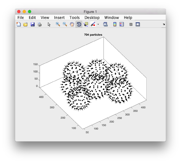
dtplot(tAll,'pf','oriented_positions');axis equal
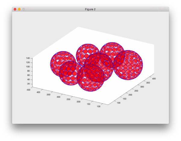
There are several programs to depict tables. In this case we may find dpktbl.plot.disks useful, as it allows to depict the particles in a table with an associated extent. This is useful to check how a given sidelength in pixels covers the vesicles for a given particle distribution.
dpktbl.plots.disks(tAll,'r',10);
Create a data folder
We can now create our typical data folder with dtcrop with a single command.
targetFolder = 'testData';
sidelength = 40;
check = dtcrop(ds.cvolume.file,tAll,targetFolder,sidelength);
Note that that dtcrop will create a new file that contains only the particles that were actually cropped from the tomogram. Some particles were probably excluded if they were too close to the boundary of the tomogram. We can read this table file into memory.
finalTable = dread([targetFolder,'/crop.tbl']);
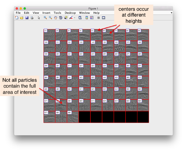
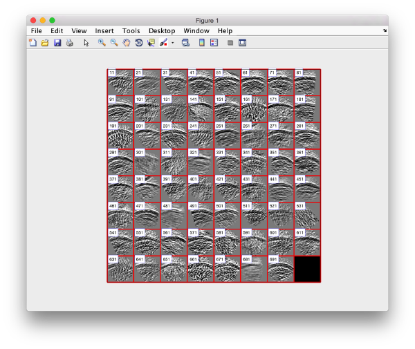
Checking the particles can be done with the interactive browsers ddbrowse or dgallery, but for a quick check we can use the dslices command:
dslices(targetFolder,'projy','*','t',finalTable,'align',1,'tag',1:10:700,'labels','on');
Here, we selected only one every ten tags to get a general idea on what is going on. The flag 'projy','*' creates a projection of the aligned particles along y, projecting all the slides, so that we can check that we are indeed greping the capsides.
We see that there are different problems: we are not hitting the center of the region of interest in many particles, and in some particles the region is out of scope.
Create a coarse average
We create a "coarse average" by just averaging all the particles with the orientations from the table, i.e, just the normals.
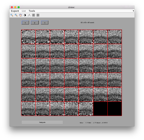
oa = daverage(targetFolder,'t',finalTable,'fc',1);
We can quickly check the result through:
dview(oa)
In this case, the area of interest is probably too low in the direction 'z': the upper half of the average is occupied by buffer. We want to lift the cropping point of the particles a little bit "downwards", that is, in the negative normal direction.
Recropping the particles
Well, the protocol that we have described step by step in the previous steps can actually be completed with a single command: the method getTableFromEnclosingSpheres
A complete syntax description can be found it:
help dmodels.dipoleSet.getTableFromEnclosingSpheres
We just want to extract a data folder where the particles are better centered and have bit more of space, so that particles stamming from spheres that are poorly defined still have a chance to get driven by a posterior alignment to the center of the box. If we initialize some variables:
sep    = 20; % for 'separation' flag. This is the separation between particles
cdfs   = -12; % for 'crop_distance_from_surface' flag, in pixels
df     = 'centeredData'; % for 'dataFolder' flag. It is the data folder were the particles will be created.
sidelength = 64;
the full task can be completed in one step:
[tnew,og] = ds.getTableFromEnclosingSpheres('sep',sep,'cdfs',cdfs,'df',df,'s', sidelength,'average',1,'mw',2);
Here the mw flag just calls for 2 cores to carry the average. If you don't have a license for the Parallel Toolbox, simply don't use the flag.
Also, notice that two outputs are produced. The first one is just the table, (including also excluded particles!). The second one includes a more detailed output, including a field averageOutput that corresponds to the output of the average operation on the newly created data folder centeredData. You can view it with the normal dview command:
dview(og.averageOutput.average);
Alignment project
The particles can now be aligned using the table and template that we just defined. We just need to write them into files
dwrite(dread([df,'/crop.tbl']),'centered.tbl');
and the density map hidden in the output:
dwrite(og.averageOutput.average,'centered.em');
and create a project
pr = 'pcnt'; % pr is a variable, "pcnt" is a literal string
We create an empty project pointing to the right data, template and table:
dcp.new(pr,'d',df,'t','centered.tbl','template','centered.em','masks','default','show',0);
Putting the 'show' flag to zero prevented the dcp GUI from popping up, as we want to use this walkthrough as an example of how to create and manage projects from the command line. The basic tool is dvput, which is used to change one or several project parameters. A list of the parameters and their syntax can be printed with dvhelp or consulted through the GUI dhelp. For this particular project we suggest the set below:
dvput(pr,'ite_r1',4);
dvput(pr,'dim_r1',32);
In the stage of finding general orientations and coarse centerings, we want to save computing time (without trading accuracy). Thus, we use the 'dim_r1' parameters tune to 32. As the particle boxes have a sidelength of 64 pixels, here we are asking Dynamo to bin each particle on the fly, just one time. A neighboorhod of 2x2x2 voxels will collapse into one single voxel, with the averaged intensity. By now, we are just interested in coarsely locating the particles, so that the speed-up in the alignemnt (8x) justifies the loss of accuracy.
Next, we need angular settings reflect that we trust the normals that we have found. This will save computation time and make the alignment more robust.
dvput(pr,'cr_r1',40);
dvput(pr,'cs_r1',20);
dvput(pr,'ir_r1',360);
dvput(pr,'is_r1',40);
dvput(pr,'rf_r1',4);
dvput(pr,'rff_r1',2);
We let the particles shift, but not the the edges of the box:
dvput(pr,'lim_r1',[20,20,20]);
dvput(pr,'limm_r1',1);
Some parameters re provided to control the execution. For projects to be run in parallel under Matlab, we need the 'destination' parameter tuned to value 'matlab_parfor'. We also provide a value for the number of cores to be used during the alignments (parameter 'cores') and the averaging steps (parameter matlab_workers_average).
dvput(pr,'dst','matlab_parfor','cores',2,'mwa',2);
Run project
As we would do the GUI, we have to check, unfold and run the project:
dvcheck pcnt
dvunfold pcnt
dvrun pcnt
In scripted protocols
Advanced: A note for future projects: when your own scripts to run several projects created dynamically, you can put the name of the project into a variable (as we did above) and use the ( )  notation:
dvcheck(pr);
dvunfold(pr);
dvrun(pr);
When used inside a script, you probably want to use the ; at the end of each line, to prevent flooding the screen with output.
Check results
We can check how the particles look like:
dslices('pcnt:data','projy','*','t','pcnt:rt:ite=3','align',1,'tag',1:10:700,'labels','on');
Here, 'pcnt:data' is a database query. it is just a shorthand to tell Dynamo to use the data folder associated with the project pcnt. The same trick is used to extract the refined table (rt) at iteration 3. Don't worry if you don't like this notation: you can just input the actual folder and file names.
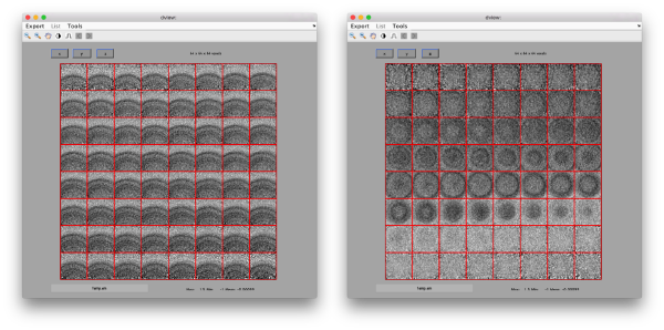
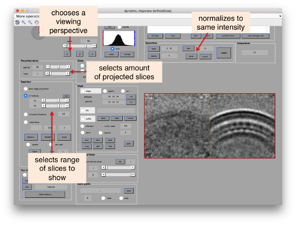
The averages can be consulted with mapview. We open the averages (a item) corresponding to iterations 0 and 4:
dpkdev.legacy.dynamo_mapview('pcnt:a:ite=[0,4]')
You can tweak the visualization to see a depiction of how the average evolved from the first template to iteration number 4.
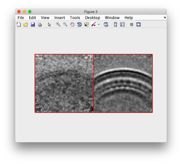
As a tip, when you know exactly which features you want to test visually, you can use the command line order dslices to directly produce the scene of interest:
dslices pcnt:a:ite=[0,4] -projy 44 -ns 1
Recropping the particles
You can create a new table excluding particles that are too close to each other:
tc = dpktbl.exclusionPerVolume('pcnt:rt:ite=4',15,22);
where 15 is a distance in pixels. The third parameter denotes the column in the table that denotes particles in the same objects. In this case, we have marked each virus with a different integer in column 22 of the table, and we pass this information to dpktbl.exclusionPerVolume.
