Difference between revisions of "Advanced starters guide"
| (103 intermediate revisions by 3 users not shown) | |||
| Line 1: | Line 1: | ||
| + | [[Category:Walkthroughs]] | ||
| − | This walkthrough uses a small size example based on a real tomogram to | + | This walkthrough uses a small size example based on a real tomogram to cover several tasks. |
| − | |||
== The example data set == | == The example data set == | ||
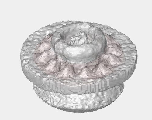
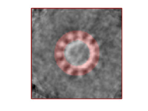
| − | The data is a fraction of a tomogram. The full tomogram was used in "Cryo-electron tomography reveals novel features of a viral RNA replication compartment." (Ertel et al.), and represents several FHV viruses docked in the membrane of a | + | The data is a fraction of a tomogram. The full tomogram was used in "Cryo-electron tomography reveals novel features of a viral RNA replication compartment." (Ertel et al.), and represents several FHV viruses docked in the outer membrane of a mitochondrion. |
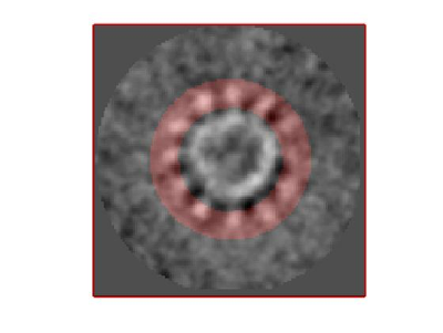
| + | [[File:FhvDefinitionCrown.png|thumb|center|500px| Average for several hundreds of particles. The "crown" area is shown under a red shadow.]] | ||
== Downloading == | == Downloading == | ||
| − | + | During the Dynamo workshop you will find the needed tilt series in your data folder. Outside the workshop, you can download all the files related to this example with the command: | |
| − | + | <tt>dpkhelp.wiki.downloadExample('fhv');</tt> | |
If it fails under Matlab or the ''Dynamo'' command line, you can try to directly use the linux order | If it fails under Matlab or the ''Dynamo'' command line, you can try to directly use the linux order | ||
<tt>wget https://wiki.dynamo.biozentrum.unibas.ch/w/doc/data/fhv/crop.rec </tt> | <tt>wget https://wiki.dynamo.biozentrum.unibas.ch/w/doc/data/fhv/crop.rec </tt> | ||
| + | |||
or | or | ||
| + | |||
<tt>curl -O https://wiki.dynamo.biozentrum.unibas.ch/w/doc/data/fhv/crop.rec </tt> | <tt>curl -O https://wiki.dynamo.biozentrum.unibas.ch/w/doc/data/fhv/crop.rec </tt> | ||
| − | |||
| − | This should have created the file called <tt>crop.rec</tt> in your current directory. | + | under MacOS. This should have created the file called <tt>crop.rec</tt> in your current directory. |
===Size check of a file=== | ===Size check of a file=== | ||
| Line 34: | Line 36: | ||
size: 1285 x 956 x 786</nowiki> | size: 1285 x 956 x 786</nowiki> | ||
| − | So, it's a tomogram. | + | So, it's a tomogram. |
| + | |||
===Lightweight visualization=== | ===Lightweight visualization=== | ||
We can inspect quickly its contents with [[Viewing_tomograms#dtmshow | dtmshow]] | We can inspect quickly its contents with [[Viewing_tomograms#dtmshow | dtmshow]] | ||
| Line 44: | Line 47: | ||
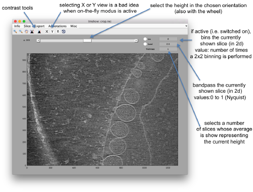
[[File:FhvTomoshowOnTheFly.png|thumb|center|500px|Basic controls of <tt>dtmshow</tt>]] | [[File:FhvTomoshowOnTheFly.png|thumb|center|500px|Basic controls of <tt>dtmshow</tt>]] | ||
| − | Go up and down. We want to select the locations were the vesicles intersect the | + | Go up and down. We want to select the locations were the vesicles intersect the mitochondrion membrane and average them together. For this, we need to ''catalogue'' the tomogram, so that our annotations are stored with a clear relationship with the tomogram. |
== Cataloguing the tomogram == | == Cataloguing the tomogram == | ||
| Line 50: | Line 53: | ||
We can create catalogues just to contain a single tomogram. They are useful to keep track of all annotations, and of the typical transforms (binning, cropping of fractions) that we usually perform on a larged size tomogram of interest. In this case, we can create the catalogue directly from the command line: | We can create catalogues just to contain a single tomogram. They are useful to keep track of all annotations, and of the typical transforms (binning, cropping of fractions) that we usually perform on a larged size tomogram of interest. In this case, we can create the catalogue directly from the command line: | ||
| − | <tt | + | <tt> dcm -create fhv </tt> |
where <tt>dcm</tt> is the short form of <tt>dynamo_catalogue_manager</tt> and <tt>fhv</tt> is just an arbitrary name. The just created catalogue is empty, and we can add our tomogram with: | where <tt>dcm</tt> is the short form of <tt>dynamo_catalogue_manager</tt> and <tt>fhv</tt> is just an arbitrary name. The just created catalogue is empty, and we can add our tomogram with: | ||
| Line 68: | Line 71: | ||
=== Prebinning the tomograms === | === Prebinning the tomograms === | ||
| − | We typically want to [[prebinned tomograms | prebin]] the tomogram, i.e., have a version of smaller size that is known to the catalogue. This version will be useful in some operations that require a full tomogram in memory, an operation that can consume much memory and need a long time. In this example, this | + | We typically want to [[prebinned tomograms | prebin]] the tomogram, i.e., have a version of |smaller size that is known to the catalogue. This version will be useful in some operations that require a full tomogram in memory, an operation that can consume much memory and need a long time. In this example, this would not be necessary: a tomogram with a sidelength on x and y of ~1000 pixels shouldn't pose any visualization problem. We do it anyway for the exercise with the command: |
<tt>dynamo_catalogue_bin('fhv', 1, 'zchunk', 300); </tt> | <tt>dynamo_catalogue_bin('fhv', 1, 'zchunk', 300); </tt> | ||
| Line 76: | Line 79: | ||
=== Operation with GUI=== | === Operation with GUI=== | ||
| − | These steps could have been performed | + | These steps could have been performed thorough the <tt>dcm</tt> GUI |
| − | |||
== Annotation of particle positions == | == Annotation of particle positions == | ||
Now we can open the tomogram through the catalogue: | Now we can open the tomogram through the catalogue: | ||
<tt>dtmslice crop.rec -c fhv -prebinned 1 </tt> | <tt>dtmslice crop.rec -c fhv -prebinned 1 </tt> | ||
| − | |||
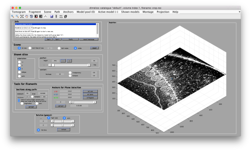
[[File:FhvTomosliceOpen.png|thumb|center|500px|dtmslice opened on the FHV example tomogram<tt>dtmslice</tt>]] | [[File:FhvTomosliceOpen.png|thumb|center|500px|dtmslice opened on the FHV example tomogram<tt>dtmslice</tt>]] | ||
| − | |||
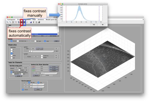
Probably you don't like the initial contrast, change it with the button in the toolbar. | Probably you don't like the initial contrast, change it with the button in the toolbar. | ||
| Line 93: | Line 93: | ||
=== Navigating the tomogram === | === Navigating the tomogram === | ||
| − | + | * left click and drag the slice with your mouse to move it up and down | |
| + | * this can also be achieved with the controls on the left hand side | ||
| + | * ctrl + left click and drag will change your viewpoint of the 3d scene | ||
| + | * shift + left click and drag will move the center of rotation | ||
| + | * ctrl + mouse wheel up/down will zoom in or out of the scene | ||
| + | |||
| + | Other [[Dtmslice#Viewing controls | axiliary tools]] are the keys x,y,z to change the slice orientation, the number of projected slices (called "thickness" in the GUI controls), the transparency of the slice. | ||
| + | |||
| + | You can reset the scene at any time by hitting the reset button. | ||
| + | |||
| + | You can save slices for viewing later with the s key. | ||
=== Creation of models to contain annotations=== | === Creation of models to contain annotations=== | ||
| Line 101: | Line 111: | ||
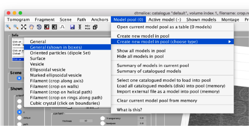
[[File:FhvBoxesModel.png|thumb|center|500px|Creating a new model in the scene. Each annotation is represented by a box]] | [[File:FhvBoxesModel.png|thumb|center|500px|Creating a new model in the scene. Each annotation is represented by a box]] | ||
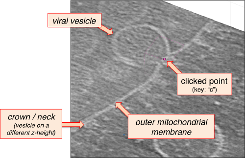
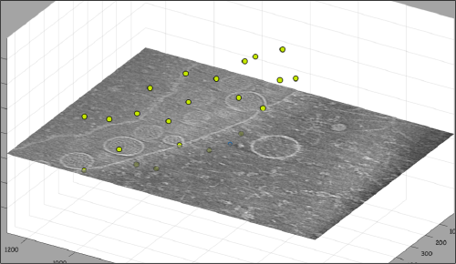
| − | After creating the model, it will be only model currently active in the <tt>dtmslice</tt> scene. You can add new points pressing on [c]. The idea is to mark on the positions where you see the "neck" of a vesicle (what we called "crowns") in contact with the | + | After creating the model, it will be only model currently active in the <tt>dtmslice</tt> scene. You can add new points pressing on [c]. The idea is to mark on the positions where you see the "neck" of a vesicle (what we called "crowns") in contact with the outer mitochondrial membrane. |
| − | [[File: | + | [[File:FhvCloseUp.png|thumb|center|500px|Clicking the crowns on screen]] |
| − | The last marked point can be deleted by pressing [delete]. An arbitrary point can be | + | The last marked point can be deleted by pressing [delete]. An arbitrary point can be deleted by clicking on it with the auxiliary mouse button. This will open a menu that includes the option of deleting the point (through Ctrl+X in Linux or Cmmd+X in Mac). |
At this stage you probably want to change the transparence of the depicted slice, so that you can control which objects have been already clicked below the depicted slide. | At this stage you probably want to change the transparence of the depicted slice, so that you can control which objects have been already clicked below the depicted slide. | ||
| Line 115: | Line 125: | ||
== Cropping particles == | == Cropping particles == | ||
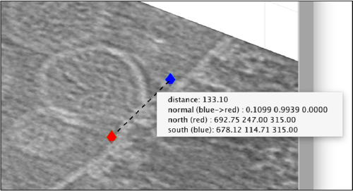
| − | Now we want to use the positions that we have marked to extract the subtomograms and format them as a [[data folder]]. The first thing we | + | Now we want to use the positions that we have marked to extract the subtomograms and format them as a [[data folder]]. The first thing we need is an estimation of the sidelength in pixels of each of the subtomograms. In [[dtmslice]] We can use the keys [1] and [2] to define two anchor points that appear as rombohedra. Clicking (with the right button) onto the black dashed that links the will show on screen both coordinates and the distance between them. All distances are reported in pixels of the non-binned tomogram: even if you are using a binned version, ''Dynamo'' keeps track of it. |
[[File:FhvMeasureDistance.png|thumb|center|500px|Measuring distances with [1] , [2] and right-click]]. | [[File:FhvMeasureDistance.png|thumb|center|500px|Measuring distances with [1] , [2] and right-click]]. | ||
| Line 126: | Line 136: | ||
Volume 1 contains 1 models in total | Volume 1 contains 1 models in total | ||
/Users/casdanie//fhv/tomograms/volume_1/models/mboxes.omd</nowiki> | /Users/casdanie//fhv/tomograms/volume_1/models/mboxes.omd</nowiki> | ||
| + | |||
| + | In your system, instead of <tt>/Users/casdanie/</tt> you will see the path to the folder where you created the catalogue <tt>fhv</tt> | ||
=== Creating a table === | === Creating a table === | ||
| − | We could just use the catalogue GUI to extract the particles, be it is also possible | + | We could just use the catalogue GUI to extract the particles, be it is also possible to proceed directly with the command line. We will use the <tt>dtcrop</tt> command, .which requires preparing a [[table]] with the information of the model. |
| − | <nowiki> | + | <nowiki>m = dread('/Users/casdanie/fhv/tomograms/volume_1/models/mboxes.omd'); |
t = m.grepTable();</nowiki> | t = m.grepTable();</nowiki> | ||
| Line 136: | Line 148: | ||
Note that we can extract models directly from the output of <tt>dcmodels</tt> | Note that we can extract models directly from the output of <tt>dcmodels</tt> | ||
| − | <nowiki> | + | <nowiki>dcmodels fhv -i 1 -ws o; |
m = dread(o.files{1}); | m = dread(o.files{1}); | ||
t = m.grepTable();</nowiki> | t = m.grepTable();</nowiki> | ||
| − | i.e., we load the answer of <tt>dcmodels</tt> for volume index <tt>-i 1</tt>in the output variable <tt>o</tt> . Inside it, there is a field called <tt>'files'</tt> which contains a [[matlab cell array| cell array]] of files containing models. Then we read the first entry <tt>o.files{1}</tt>. | + | i.e., we load the answer of <tt>dcmodels</tt> for volume index <tt>-i 1</tt> in the output variable <tt>o</tt>. Inside it, there is a field called <tt>'files'</tt> which contains a [[matlab cell array| cell array]] of files containing models. Then we read the first entry <tt>o.files{1}</tt>. |
Whichever way you create the table variable <tt>t</tt>, it is just a matrix with a row for each particle, and a summary of the information coded inside can be created through: | Whichever way you create the table variable <tt>t</tt>, it is just a matrix with a row for each particle, and a summary of the information coded inside can be created through: | ||
| − | < | + | <nowiki>>> dtinfo(t); |
size : 22 35 | size : 22 35 | ||
| Line 174: | Line 186: | ||
[ 37 ] defocus : Warning: column not available in this table</nowiki> | [ 37 ] defocus : Warning: column not available in this table</nowiki> | ||
| − | === Using dtcrop === | + | === Using <tt>dtcrop</tt> === |
| − | The simplest syntax of <tt>dtcrop< | + | The simplest syntax of <tt>dtcrop</tt> requires passing the name of the tomogram from which we want to crop (syntax varies for [[ Particle extraction#Extract from different tomograms| cropping from multiple tomograms]]). We know that the file is <tt>crop.rec</tt>, and we could directly insert this name in the command. But a catalogued model already contains information about its source tomogram (inside its property <tt>cvolume</tt>), so that we can always track it back. We could then define a variable <tt>tomogramFile</tt> by accessing this information inside the model variable <tt>m</tt>: |
<tt>tomogramFile = m.cvolume.file();</tt> | <tt>tomogramFile = m.cvolume.file();</tt> | ||
| − | + | if you get a warning at this stage, don't worry, the command still worked. | |
| + | |||
| + | You can then launch the cropping order: | ||
| + | |||
<tt>o = dtcrop(tomogramFile,t,'particlesData',128);</tt> | <tt>o = dtcrop(tomogramFile,t,'particlesData',128);</tt> | ||
where you could add the <tt>mw</tt> flag to let ''Dynamo'' use several cores. In any case, for this number or particles the cropping should take some seconds. The last part of the final output into screen should look like this: | where you could add the <tt>mw</tt> flag to let ''Dynamo'' use several cores. In any case, for this number or particles the cropping should take some seconds. The last part of the final output into screen should look like this: | ||
| − | <nowiki> | + | <nowiki>21 [read_subtomogram] Volume has size 1285 956 786 |
| − | 21 [read_subtomogram] Volume has size 1285 956 786 | ||
[read_subtomogram] Accessing subvolume x: 713:840; y: 339:466; z: 160:287 totalling ~ 16.0Mb | [read_subtomogram] Accessing subvolume x: 713:840; y: 339:466; z: 160:287 totalling ~ 16.0Mb | ||
Elapsed time is 0.191014 seconds. | Elapsed time is 0.191014 seconds. | ||
| Line 199: | Line 213: | ||
informing you that some of the particles where excluded, as they were probably too close to the boundary of the tomogram, given the sidelength we asked for. Inside the created data folder, | informing you that some of the particles where excluded, as they were probably too close to the boundary of the tomogram, given the sidelength we asked for. Inside the created data folder, | ||
| − | + | you will find the table <tt>particlesData/crop.tbl</tt>, which only indexes the actually cropped particles. | |
| − | |||
=== Creating an average === | === Creating an average === | ||
| Line 208: | Line 221: | ||
<tt>oa = daverage('particlesData','t','particlesData/crop.tbl');</tt> | <tt>oa = daverage('particlesData','t','particlesData/crop.tbl');</tt> | ||
| − | If you want to let ''Dynamo'' pass maps into Chimera, you have to inform ''Dynamo'' on the location of Chimera. | + | If you want to let ''Dynamo'' pass maps into Chimera, you have to inform ''Dynamo'' on the location of Chimera. For instance: |
| − | <tt>dchimera - | + | |
| + | <tt>dchimera -setPath /usr/local/bin/ </tt> | ||
| + | |||
| + | Please adapt it to the location of Chimera in your file system. | ||
| + | |||
| + | To open your average in chimera | ||
| + | |||
| + | <tt> dchimera(oa.average) </tt> | ||
== Project to find membrane orientations== | == Project to find membrane orientations== | ||
| Line 219: | Line 239: | ||
We can create a project directly thorugh the command line: | We can create a project directly thorugh the command line: | ||
| − | <tt>dcp.new('first','d','particlesData','template | + | <tt>dcp.new('first','d','particlesData','template','rawTemplate.em','masks','default','t','particlesData/crop.tbl');</tt> |
...and go directly to the panel of numerical parameters to create a project adapted for catching the general orientation of the membrane: | ...and go directly to the panel of numerical parameters to create a project adapted for catching the general orientation of the membrane: | ||
[[File:FhvFirstParameters.png|thumb|center|500px| Numerical parameters for just membrane orientation]] | [[File:FhvFirstParameters.png|thumb|center|500px| Numerical parameters for just membrane orientation]] | ||
| − | <tt> | + | |
| − | < | + | Also, remember to visit the window for execution environment, and select the appropriate settings. If you are working with Matlab, select ''Matlab''(for one single core) or "Matlab_parfor" (if you are going to several cores). If working with the standalone, use the [[standalone]] option. In both cases, select the number of cores for alignment (green box in the picture below) and averaging (blue box) . |
| − | + | ||
| − | + | [[File:FhvEnvironment.png|thumb|center|500px| Selecting the execution modus]] | |
| + | |||
| + | You can operate the project management operations from the GUI or the command line. First checking: | ||
| + | |||
| + | <tt>dvcheck first</tt> | ||
| + | |||
| + | then unfolding | ||
| + | |||
| + | <tt>dvunfold first</tt> | ||
| + | |||
| + | and finally running it by invoking the name of the execution script. If you are running in Matlab use: | ||
| + | |||
| + | <tt>first</tt> | ||
| + | |||
| + | If you are running ''Dynamo'' in standalone modus, open a new tab (or window) of the terminal, load Dynamo (but don't run Dynamo) and type: | ||
| + | |||
| + | <tt>./first.exe</tt> | ||
After running the project, we check the created average: | After running the project, we check the created average: | ||
| Line 234: | Line 270: | ||
This command asks the database (hence <tt>db</tt>) of the project <tt>first</tt> to look for the item of type <tt>average</tt>, by default accessing the last computed one. The flag <tt>-v</tt> sends the output of the database query to the depiction GUI called <tt>dview</tt>. | This command asks the database (hence <tt>db</tt>) of the project <tt>first</tt> to look for the item of type <tt>average</tt>, by default accessing the last computed one. The flag <tt>-v</tt> sends the output of the database query to the depiction GUI called <tt>dview</tt>. | ||
| − | [[File:FhvFirstAverage.png|thumb|center|500px|First average, no | + | [[File:FhvFirstAverage.png|thumb|center|500px|First average, no azimuthal rotation was tested. Shown in <tt> dview</tt> program]] |
Apparently, the project finds the membranes and centers the particles correctly. If you show the volume in Chimera (by clicking in the ''Export>Send to Chimera'' option in the <tt>dview</tt> window ). | Apparently, the project finds the membranes and centers the particles correctly. If you show the volume in Chimera (by clicking in the ''Export>Send to Chimera'' option in the <tt>dview</tt> window ). | ||
| − | [[File:FhvFirstChimera.png|thumb|center|500px|First average, no | + | [[File:FhvFirstChimera.png|thumb|center|500px|First average, no azimuthal rotation was tested ]] |
We can check the individual particles: | We can check the individual particles: | ||
| Line 248: | Line 284: | ||
== Aligning the axis of symmetry == | == Aligning the axis of symmetry == | ||
| − | We would like to bring the axis of symmetry to the ''z''direction. This will create an intuitive separation between the two first euler angles that represent "change of orientation of the main axis", and the third one that represents " | + | We would like to bring the axis of symmetry to the ''z''direction. This will create an intuitive separation between the two first euler angles that represent "change of orientation of the main axis", and the third one that represents "azimuthal rotation about the new axis". We want that azimuthal rotations occur about an axis of possible symmetry, which by convention is located along z. There are several ways to achieve this. A simple one is to create a model of the membrane/crown geometry, align our average to it (with <tt>dalign</tt>), and use the alignment parameters to create a new table. With this new table and average we will be able study possible symmetries with a new project. |
| Line 257: | Line 293: | ||
<nowiki>mr = dpktomo.examples.motiveTypes.MembraneWithRod(); | <nowiki>mr = dpktomo.examples.motiveTypes.MembraneWithRod(); | ||
mr.sidelength = 128; | mr.sidelength = 128; | ||
| − | mr.rodRadius = 20; mr.rodShift = [0,0,10];mr.rodHeight= | + | mr.rodRadius = 20; mr.rodShift = [0,0,10]; mr.rodHeight= 20; |
mr.getMask(); | mr.getMask(); | ||
template = mr.mask;</nowiki> | template = mr.mask;</nowiki> | ||
| + | |||
| + | Note that you can check the list of properties inside the object <tt>mr</tt> just by typing it without the semicolon and pressing [Return] | ||
We can check the result with: | We can check the result with: | ||
| − | <tt>mr.viewMask();</tt> | + | <tt>mr.viewMask();</tt> |
| − | |||
[[File:FhvTemplateZ.png|thumb|center|700px| A simple template with rotational symmetry axis aligned along z]] | [[File:FhvTemplateZ.png|thumb|center|700px| A simple template with rotational symmetry axis aligned along z]] | ||
| − | |||
=== Aligning the previous average along z === | === Aligning the previous average along z === | ||
| − | The mask is white on black by definition. The tomogram data in this case represents bright protein on dark background, so that in this case we want to align the previously | + | The mask is white on black by definition. The tomogram data in this case represents bright protein on dark background, so that in this case we want to align the previously computed average to the mask of the <tt>mr</tt> object. |
| − | The alignment does not need to scan | + | The alignment does not need to scan azimuthal rotations, so that our 'inplane_range' will be 0. The 'cone_range' will be the full sphere, and we take and spacing of 30 degrees. As we are looking for coarse orientations, we can bin the two volumes twice (yielding volumes with a sidelength of 32 pixels). We will also "nail" the new center to the physical center of the box (parameter <tt>limm</tt> set to 1 below). |
Now we read the average computed by the project <tt>first</tt> into a workspace variable which we arbitrarily call <tt>previousAverage</tt> | Now we read the average computed by the project <tt>first</tt> into a workspace variable which we arbitrarily call <tt>previousAverage</tt> | ||
| − | <tt>ddb first:a -r | + | <tt>ddb first:a -r previousAverage;</tt> |
| − | <tt>previousAverage</tt> | + | Here, the volume <tt>previousAverage</tt> will be treated as a "particle" to be aligned onto a ''template'', which in this case is the volume contained in <tt>mr.mask</tt>. |
| − | <tt>sal = dalign(previousAverage,mr.mask,'cr',360,'cs',30,'ir',0,'dim',32,'limm',1,'lim',[10,10,10]); </tt> | + | |
| + | <tt>sal = dalign(previousAverage,mr.mask,'cr',360,'cs',30,'ir',0,'dim',32,'limm',1,'lim',[10,10,10]); </tt> | ||
The flags are the same parameters that would be used in an alignment project. You can check the shorthands with <tt>dvhelp</tt>. | The flags are the same parameters that would be used in an alignment project. You can check the shorthands with <tt>dvhelp</tt>. | ||
| − | The output result <tt>sal</tt> contains many fields. We can, for instance directly visualize how the previous average looks like when transformed through the results of this <tt>dalign</tt> operation. | + | The output result <tt>sal</tt> contains many fields. We can, for instance directly visualize how the previous average looks like when transformed through the results of this <tt>dalign</tt> operation. For this, use the field <tt>aligned_particle</tt> in the output <tt>sal</tt>: |
| + | |||
| + | <tt>dview(sal.aligned_particle);</tt> | ||
| + | |||
| + | |||
[[File:ZAlignedAverage.png|thumb|center|700px| A simple template with rotational symmetry axis aligned along z]] | [[File:ZAlignedAverage.png|thumb|center|700px| A simple template with rotational symmetry axis aligned along z]] | ||
| Line 294: | Line 335: | ||
The variable <tt>tf </tt> contains now the original table, which is now rotated and shifted according with the rigid body transform <tt>Tp</tt> inside <tt>sal</tt> | The variable <tt>tf </tt> contains now the original table, which is now rotated and shifted according with the rigid body transform <tt>Tp</tt> inside <tt>sal</tt> | ||
| − | <tt> | + | <tt>tr = dynamo_table_rigid(tf,sal.Tp); </tt> |
| − | now <tt> | + | now the ''rectified ''table <tt>tr</tt> should contain the metadata that makes the particles "point upward". We use now the typical sanity check to assess that a table behave as expected: we apply it to the particles in its paired [[data folder]] and check the average: |
| − | + | ||
| + | <tt>oz = daverage('first:data','t',tr,'fc',1); </tt> | ||
whose results can be checked by: | whose results can be checked by: | ||
| − | <tt>dview( | + | <tt>dview(oz); </tt> |
| + | |||
| + | [[File:FhvSanityCheckZ.png|thumb|center|700px| Particles aligned with rectified table <tt>tr</tt>]] | ||
| + | |||
| + | |||
| + | We can visualize this operation by plotting a sketch with the orientation of the particles. We first show the results for the table computed in the project <tt>first</tt> | ||
| + | |||
| + | <nowiki>figure; | ||
| + | dtplot('first:rt','m','sketch','sketch_length',100,'sm',30); | ||
| + | view(-230,30);axis equal;</nowiki> | ||
| + | |||
| + | [[File:FhvSketchFirst.png|thumb|center|400px| sketch of orientations after computation of the the project <tt>first</tt>]] | ||
| + | |||
| + | Here, the 'z' orientation computed for each particle is represented by the longest semiaxis. Note that with the original definition of the template, the 'z' points -approximately- along the direction of the 'z' in the tomogram. If we depict the same plot with the table we just computed: | ||
| + | |||
| + | <nowiki>figure; | ||
| + | dtplot(tr,'m','sketch','sketch_length',100,'sm',30); | ||
| + | view(-230,30);axis equal;</nowiki> | ||
| + | |||
| + | [[File:FhvSketchZ.png|thumb|center|400px| sketch of orientations in the rectified table]] | ||
| + | |||
| + | we see that now the 'z' axis in each particle is pointing orthogonally(-ish) to the membrane. A different quick check would be to show the projections of the particles along ''y''. Instead of using the GUI <tt>ddbrowse</tt>, we can create this depiction with a single command: | ||
| + | |||
| + | <tt>figure;dslices('particlesData','t',tr,'projy','*','align',1,'labels','on'); </tt> | ||
| + | |||
| + | [[File:fhvOrientedSlicesX.png|thumb|center|400px| full ''y''projection of the particles according to the orientations in the rectified table ]] | ||
| + | |||
| + | Lets look at the ''z''-projection. In this case we project only the central slices around the crown and the aperture in the viral vesicle, chosing thus slices 60 to 70. if project the full particle, we won't distinguish any features. | ||
| + | |||
| + | <tt>figure;dslices('particlesData','t',tr,'projz',60:80,'align',1,'labels','on');</tt> | ||
| + | |||
| + | [[File:fhvOrientedSlicesZ.png|thumb|center|400px| ''z''projection of the central slices in the rectified table ]] | ||
| + | |||
| + | The depiction clearly shows the missing wedge of the particles. Incidentally, it also shows that averaging all the particles should produce an average that covers all the orientaions in the Fourier space. | ||
| + | |||
| + | == Using the membrane to impart an orientation == | ||
| + | |||
| + | This section describes an '''alternative''' method to compute: | ||
| + | * a rough orientation of the particles, and | ||
| + | * a rough first template | ||
| + | |||
| + | In this section we will use the membrane of the mithocondrion to assign a roughly orientation to each of the points in the table. This orientation will be defined by the normal of the closest point in the membrane. The membrane will be defined as a a triangulation, to be constructed based on a set of manually picked points. | ||
| + | |||
| + | === Pick membrane points=== | ||
| + | |||
| + | We open our tomogram in <tt>dtmslice</tt> | ||
| + | |||
| + | <tt>dtmslice @{fhv}1 -prebin 1</tt> | ||
| + | |||
| + | or, if you are working with the [[standalone]] version, please prepend a "\" symbol: | ||
| + | |||
| + | <tt>\dtmslice @{fhv}1 -prebin 1</tt> | ||
| + | |||
| + | In this variant of the syntax of <tt>dtmslice</tt>, the string <tt>@{fhv}1</tt> just means "tomogram number 1 inside catalogue <tt>fhv</tt>. On the opened scene, we will use a [[Montage viewer for membrane picking | montage ]] to manually click on a set of membrane points. | ||
| + | |||
| + | '''Note! (08/06/21) - the montage viewer was recently updated and no longer provides the ability to easily add points, please define your surface model on sequential z-slices in dtmslice directly by annotating points every 20 or so slices.''' | ||
| + | |||
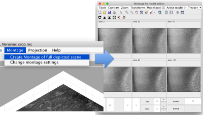
| + | [[ File:FhvMontage.png |thumb|center|400px| Opening a montage view]] | ||
| + | |||
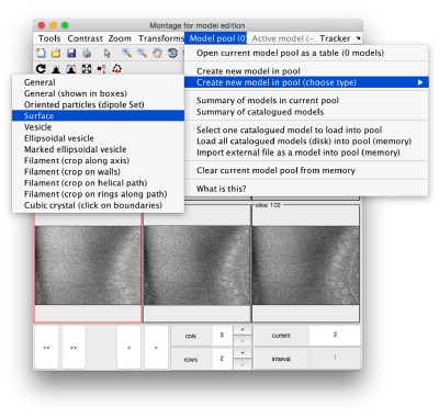
| + | By default, this <tt>montage</tt> represents slices taken orthogonally to ''z'' every 20 pixels of the unbinned tomogram. This can be changed in the settings ''before'' opening the montage GUI. Now, we can create a model of type <tt>Surface</tt>, which we will use to store a set of points in the membrane to be picked manually (or semiautomatically). To do this, go to ''Model pool> Create new model in pool (choose type) > surface '' | ||
| + | |||
| + | [[ File:FhvCreateSurfaceModel.png |thumb|center|400px| Creating a surface model]] | ||
| + | |||
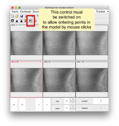
| + | You need to click on the point switcher (the control in the toolbar with a ''c'' and an ''i'') to allow entering points. The basic controls are: | ||
| + | * Mouse click to enter a point. | ||
| + | * <tt>d</tt> to delete a point. | ||
| + | * <tt>i</tt> to insert a point. | ||
| + | |||
| + | [[File:FhvMontageActiveClick.png |thumb|center|400px| Point switcher must be toggle on to pick points into the model]] | ||
| + | |||
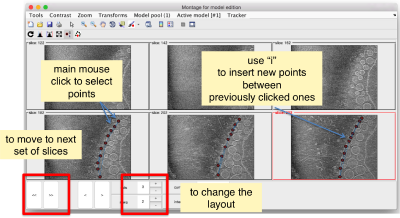
| + | Use the ''>>'' button in the bottom of the GUI to go to next set of orthoslices. | ||
| + | |||
| + | [[File:FhvMontageControls.png |thumb|center|400px| Controls of the montage GUI]] | ||
| + | |||
| + | Note that the points that you click in the Montage GUI are assigned to a model in the pool, and as such, they appear automatically in the dtmslice GUI | ||
| + | [[ File:FhvTmsliceUpdates.png |thumb|center|600px| Points clicked in the montage GUI reflect in the <tt>tmslice</tt> GUI]] | ||
| + | |||
| + | You also need <tt>shift + C </tt> in order to place a center inside the mithocondrion. This point is just used to tell ''Dynamo'' what is the inside and what is the outside face of the surface that we are building. | ||
| + | |||
| + | [[File:FhvSurfaceMarkCenter.png |thumb|center|400px| <tt>shift + C </tt> marks an arbitrary interior point]] | ||
| + | |||
| + | ==== Automatic detection ==== | ||
| + | |||
| + | Once you have clicked points on a level, you can try and check if the automatic tracker can locate them in the next one. To do so, activate the next slice (i.e., secondary click it, so that its frame becomes red), and press <tt>o</tt>. You can edit the points with <tt>d</tt> to delete the closest point, <tt>m</tt> to move the closest point to the position currently under the cursor, or <tt>l</tt> to delete all the points detected in the slice... in such a case, you probably want to check the tracking parameters before using <tt>o</tt> again! | ||
| + | |||
| + | === Create a surface === | ||
| + | |||
| + | Now, we want to convert the points that we have introduced into a triangulation. This is a part of the [[Membrane Models#Workflow description| workflow]] used to crop particles from [[membrane models]], so we open the workflow GUI for this model in the ''Active Model'' menu tab. | ||
| + | |||
| + | [[ File:FhvSurfaceWorkflowCreate.png |thumb|center|400px| Invoking the workflow editor of active model ]] | ||
| + | |||
| + | We can first check the points currently contained in the model, by auxiliary clicking on the first viewing option and choosing the ''User points'' option. They will be depicted in a graphic window which will update with the new graphical elements that we depict there. | ||
| + | |||
| + | [[ File:FhvSurfacePlotPoints.png|thumb|center|600px| Showing original points in the model workflow GUI ]] | ||
| + | |||
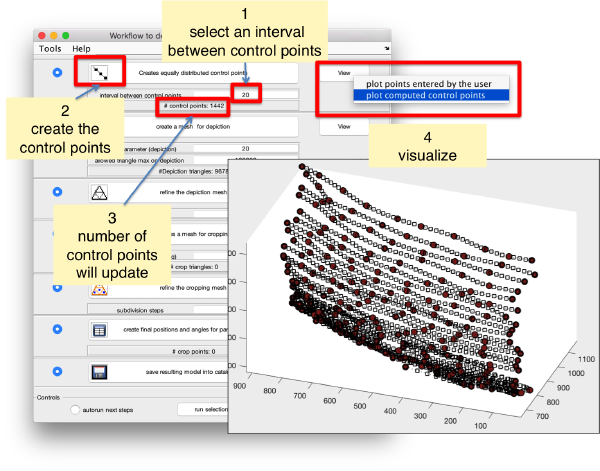
| + | We first need to create a spline interpolation on each of the levels of our point cloud. | ||
| + | |||
| + | [[ File:FhvSurfaceControlPoints.png|thumb|center|600px| Control points are created by spline interpolation. ]] | ||
| + | |||
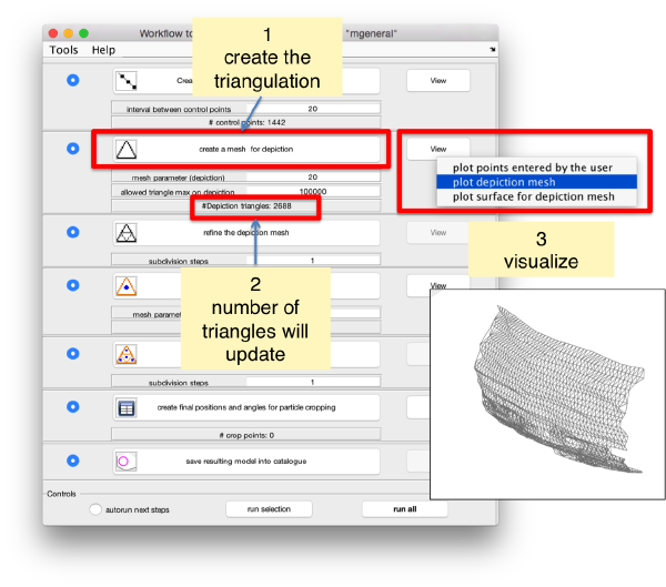
| + | Now we define a triangulation on this control points. | ||
| + | |||
| + | [[ File:FhvSurfaceCreateTriangulation.png |thumb|center|600px| Creating a triangulation on the control points ]] | ||
| + | |||
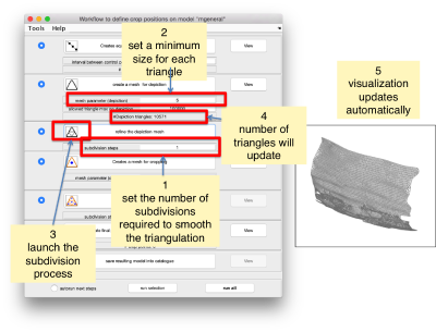
| + | Which can be subdivided to get a smoother appearance, and also a more accurate representation of the geometry. | ||
| + | |||
| + | [[File:FhvSurfaceSubdivisionMinimum.png |thumb|center|400px| A single round of subdivision smoothens the appearance of the lattice ]] | ||
| + | |||
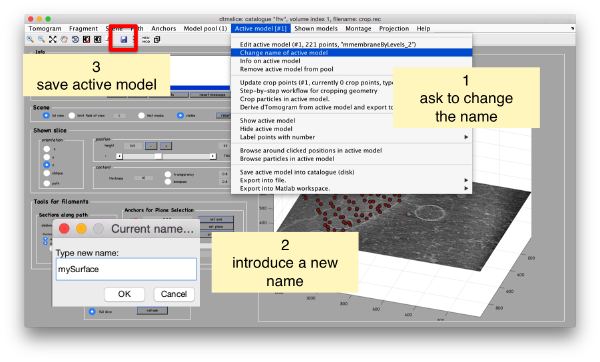
| + | Then, we can change the name of the model for clarity, and then save it into the catalogue (with the disk icon in <tt>tmslice</tt> or the ''Save into catalogue'' options under the ''Active model'' menu) | ||
| + | [[ File:FhvSurfaceSaveModel.png |thumb|center|600px| Renaming a saving a model into the catalogue ]] | ||
| + | |||
| + | === Use a surface to impart orientation === | ||
| + | |||
| + | We bring the model into our workspace. We search for it in the catalogue: | ||
| + | |||
| + | <tt>dcmodels fhv -nc mySurface -ws output</tt> | ||
| + | |||
| + | which will prompt the response | ||
| + | |||
| + | <nowiki>Volume 1. Matching models: 1 (total: 1) | ||
| + | /Users/casdanie/dynamo/examples/fhvParis/fhv/tomograms/volume_1/models/mySurface.omd</nowiki> | ||
| + | |||
| + | now, we can read the model file into our memory space to operate with it: | ||
| + | |||
| + | <tt>m = dread(output.files{1});</tt> | ||
| + | |||
| + | Now the model <tt>m</tt> is in our space of memory and can be used to impart an orientation to the points in our table. | ||
| + | |||
| + | <tt>tOrientedBySurface = dpktbl.triangulation.fillTable(m,'raw.tbl');</tt> | ||
| + | |||
| + | In this table, orientations are orthogonal to the membrane (or more precisely, orthogonal to the closest triangle in the mesh that represents the membrane) | ||
| + | |||
| + | <tt> figure;dslices('particlesData','t', tOrientedBySurface,'projy','c20','align',1,'labels','on');</tt> | ||
| + | |||
| + | [[ File:FhvMembraneSlicesPreflipping.png|thumb|center|400px| Slices along the xz plane as seen by the table]] | ||
| + | |||
| + | <tt>tConsistent = dynamo_table_flip_normals(tOrientedBySurface,'center',m.center)</tt> | ||
| + | |||
| + | We can check the effect of this table on the particles through: | ||
| + | |||
| + | <tt>figure;dslices('particlesData','t', tConsistent,'projy','c20','align',1,'labels','on');</tt> | ||
| + | |||
| + | [[ File:FhvMembraneSlicesPostflipping.png |thumb|center|400px| Slices along the xz plane as seen by the table, after using the center point to establish the interior side of the surface ]] | ||
| + | |||
| + | To get a better graphical impression, we can depict our surface (contained in the model <tt>m</tt>) with: | ||
| + | |||
| + | <tt>m.ezplot</tt> | ||
| + | |||
| + | and choose the <tt>Surface</tt>option | ||
| + | |||
| + | [[ File:FhvMembraneSurfaceEzplot.png |thumb|center|400px| Easy way to get all defined plots of a model object. ]] | ||
| + | |||
| + | Then, we just plot the positions of the particles on the same graphical figure: | ||
| + | |||
| + | <tt>dtplot(tConsistent,'m','sketch','sketch_length',100,'sm',30);</tt> | ||
| + | |||
| + | [[ File:FhvMembraneSketchDtplot.png |thumb|center|400px| <tt>dtplot</tt> directs its output on the last active figure ]] | ||
| + | |||
| + | ==== Management of the missing wedge ==== | ||
| + | |||
| + | When we create a table considering only the orientations of the points with relation to a membrane, there is no particular preference for rotations of the particles about the normal direction (i.e., azimuthal directions). The <tt>narot</tt> angle in this table is initialized to zero | ||
| + | |||
| + | Thus, take into account that an average created on these particles will have a strong missing wedge, especially in our case, where we have a preferential direction. This can be checked by averaging the particles against this table: | ||
| + | |||
| + | <tt>oa=daverage('particlesData','t', tConsistent,'fc',1);</tt> | ||
| + | Here, we ask (<tt>'fc',1</tt>) to run a Fourier compensation step, so that we can check in the output <tt>oa</tt> the property <tt>fweight</tt>, which contains the number of times a Fourier component is represented in the average. Bright values mean that the Fourier component is present in many particles (yielding thus an average of better quality for the involved frequencies). | ||
| + | |||
| + | <tt>dview(oa.fweight);</tt> | ||
| + | |||
| + | [[ File:FhvMembraneMissingWedge.png|thumb|center|400px| Fourier component presence without azimuthal randomization ]] | ||
| + | |||
| + | We can atenuate this effect by randomizing the rotational angle: | ||
| + | |||
| + | <tt>tConsistentRandomized = dynamo_table_randomize_azimuth( tConsistent);</tt> | ||
| + | |||
| + | and averaging again. | ||
| − | [[File: | + | <tt>oaRandomized=daverage('particlesData','t', tConsistentRandomized,'fc',1);</tt> |
| + | |||
| + | Now, the <tt>fweight</tt> map doesn't show such a strongly preferential orientation: | ||
| + | |||
| + | <tt>dview(oaRandomized.fweight);</tt> | ||
| + | |||
| + | [[ File:FhvMembraneMissingRandomized.png |thumb|center|400px| Fourier component presence with azimuthal randomization ]] | ||
| + | |||
| + | The effect in direct space can be shown by depicting both averages (with and without randomization side to side) | ||
| + | |||
| + | <tt>dpkdev.legacy.dynamo_mapview({oa.average,oaRandomized.average});</tt> | ||
| + | |||
| + | [[ File:FhvMembraneCompareWedges.png |thumb|center|400px| The map on the left shows a worse definition and clear traces of missing Fourier components ]] | ||
== Project for rotational alignment == | == Project for rotational alignment == | ||
| − | We | + | We have now a template and a coherently defined metadata (i.e. table) that align the particles coarsely along the right direction. We write them into disk: |
| + | <nowiki>Insert non-formatted text here</nowiki> | ||
| + | If you did not create a membrane model, use the results of the alignment project: | ||
| + | |||
| + | <nowiki>dwrite(tr,'zOriented.tbl'); | ||
| + | dwrite(oz.average,'zOriented.em');</nowiki> | ||
| + | |||
| + | If you did create a membrane model, used the corresponding table and average: | ||
| + | |||
| + | <nowiki>dwrite(tConsistentRandomized,'zOriented.tbl'); | ||
| + | dwrite(oaRandomized.average,'zOriented.em');</nowiki> | ||
| − | |||
| − | |||
and create a project with these files. Note that the [[data folder]] remains unchanged. | and create a project with these files. Note that the [[data folder]] remains unchanged. | ||
| − | <tt>dcp.new(' | + | <tt>dcp.new('zOriented','d','particlesData','template','zOriented.em','masks','default','t','zOriented.tbl');</tt> |
In this project, we will ask for a symmetrization 'c57'.. this is just to simulate fully rotational symmetry. We are not assuming that this symmetry is physical: we just want to force any possible symmetry axis in the data along the ''z'' axis. We also keep binning twice the particles, in order to get the computation times short. | In this project, we will ask for a symmetrization 'c57'.. this is just to simulate fully rotational symmetry. We are not assuming that this symmetry is physical: we just want to force any possible symmetry axis in the data along the ''z'' axis. We also keep binning twice the particles, in order to get the computation times short. | ||
| − | [[File:.png|thumb|center|500px| Alignment parameters in <tt>zOriented</tt>]] | + | [[File:FhvZOrientedParameters.png|thumb|center|500px| Alignment parameters in <tt>zOriented</tt>]] |
| − | [[File:.png|thumb|center|500px| Alignment parameters in <tt> | + | The result shown an incipient formation of the crown... however, the presence of suspicious striations in a preferential direction might be an indication of the effect of the missing wedge. |
| + | |||
| + | [[File:FhvZOrientedMapview.png|thumb|center|500px| Result in <tt>zOriented</tt>]] | ||
| + | |||
| + | == Project with rotational randomization == | ||
| + | |||
| + | We can create a template that does not have a prefererential orintation, by just randomizing the azimuthal rotations in our table, We extract the last refined table into the variable <tt>tns</tt> | ||
| + | |||
| + | <tt>ddb zOriented:rt -r tns </tt> | ||
| + | |||
| + | and impose a perturbation that keeps all other parameters constant but randomly rotates the particles around their axis | ||
| + | <tt>tr = dynamo_table_perturbation(tns,'pshift',0,'paxis',0,'pnarot',360);</tt> | ||
| + | |||
| + | We can use this table to average again the particles and check the average. | ||
| + | <nowiki>oar = daverage('particlesData','t',tr,'fc',1); | ||
| + | dview(oar)</nowiki> | ||
| + | |||
| + | Now, we can write these files in disk and create a project: | ||
| + | <nowiki>dwrite(oar.average,'randomizedAverage.em'); | ||
| + | dwrite(tr,'randomized.tbl'); | ||
| + | dcp.new('zRandomized','d','particlesData','template','randomizedAverage.em','masks','default','t','randomized.tbl');</nowiki> | ||
| + | |||
| + | [[File:FHV zRandomized Parameters.png|thumb|center|600px| Alignment parameters in <tt>zRandomized</tt> project]] | ||
| + | |||
| + | After running this projects, the presence of a crown-like is very, very faintly hinted in mapview: | ||
| + | |||
| + | <tt>dpkdev.legacy.dynamo_mapview('zRandomized:a')</tt> | ||
| + | |||
| + | [[File:FhvRandomizedFaintHintsMapview.png|thumb|center|500px| Result from <tt>zRandomized</tt> project]] | ||
| + | |||
| + | and barely identifialble in Chimera: | ||
| + | |||
| + | [[File:FhvZRandomizedChimera.png|thumb|center|500px| Alignment parameters in <tt>localized</tt> project]] | ||
== Project for localized alignment == | == Project for localized alignment == | ||
| Line 327: | Line 595: | ||
=== Creating a tight mask === | === Creating a tight mask === | ||
| + | We want to create a mask that encloses the area of interest. To do this, we open the average in <tt>dmapview</tt>: | ||
| − | + | <tt>dpkdev.legacy.dynamo_mapview('zRandomized:a')</tt> | |
| − | |||
| − | |||
We tune the browser for viewing along ''y'', and we select one of the central slices. We can use a thickness of several pixels to have a better view. | We tune the browser for viewing along ''y'', and we select one of the central slices. We can use a thickness of several pixels to have a better view. | ||
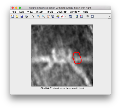
| − | + | Then, we select the area that we want to use as seed in this plane to create a revolution solid. We press on <tt>[shift] + [s] </tt> on the selected slide, letting a new window pop up. In this window, you handdraw an area on the XZ plane (main click to start drawing, auxiliary click to stop). ''Dynamo'' will rotate the region about the ''z'' axis, creating a revolution solid into the <tt>file temp_drawn_revolution_mask.em</tt> | |
| + | [[File:fhvHandDrawn.png|thumb|center|500px| Drawing a revolution mask.]] | ||
| − | + | We have to change the default name given by ''Dynamo'' to a relevant one: | |
| − | We have to change the default name given by ''Dynamo'' to | + | |
| − | <tt> !mv temp_drawn_revolution_mask.em teethMask.em </tt> | + | <tt>!mv temp_drawn_revolution_mask.em teethMask.em</tt> |
and now continue the previous project by transferring the results of <tt>zRandomized</tt> to a fresh project (lets call it <tt>localized</tt>) | and now continue the previous project by transferring the results of <tt>zRandomized</tt> to a fresh project (lets call it <tt>localized</tt>) | ||
| Line 358: | Line 626: | ||
[[File:FhvLocalizedChimera.png|thumb|center|500px| Last average in project <tt>localized</tt> as shown by <tt>mapview</tt>]] | [[File:FhvLocalizedChimera.png|thumb|center|500px| Last average in project <tt>localized</tt> as shown by <tt>mapview</tt>]] | ||
| + | |||
| + | === Testing the symmetry === | ||
| + | |||
| + | We can check for different symmetry operators to confirm the presence of symmetry. | ||
| + | |||
| + | ==== Basic command ==== | ||
| + | |||
| + | The basic command for this task is <tt>dynamo_symmetry_scan</tt>. In its fundamental syntax, you need to state the type of symmetry operator to be tested, and a set of operator. | ||
| + | |||
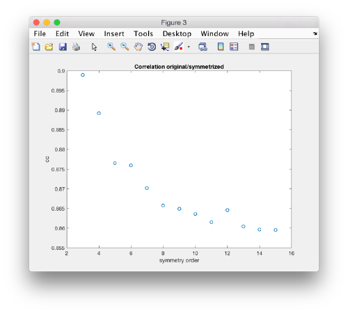
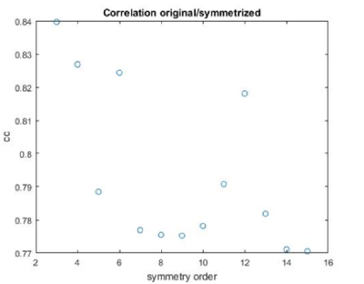
| + | <tt> stm = dynamo_symmetry_scan('localized:a','c','order',3:15,'type','pearson','nfig',3); </tt> | ||
| + | |||
| + | [[File:FhvSymmetryGlobal.png|thumb|center|500px| Symmetry detected for different masks]] | ||
| + | |||
| + | With a more localized mask: | ||
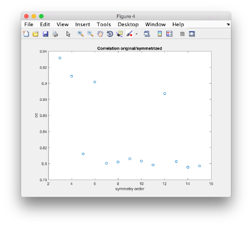
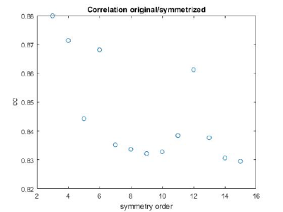
| + | <tt> slm = dynamo_symmetry_scan('localized:a','c','order',3:15,'type','pearson','mask','teethMask.em','nfig',4);</tt> | ||
| + | |||
| + | [[File:FhvSymmetryLocal.png|thumb|center|500px| Symmetry detected for different masks]] | ||
| + | |||
| + | ==== Interpretation of results ==== | ||
| + | |||
| + | If you got the results above, you might have jumped to the conclusion that they already constitute an objective hint at a real C12 symmetry. This is, however, not true. The fact is that, with a slightly different picking of particles, you could have obtained the profiles in these pictures: | ||
| + | |||
| + | {|style="margin: 0 auto;" | ||
| + | | [[File:FhvSymmetryGlobalWrong.png|thumb|upright|400px| Symmetry merit plot (global mask) ]] | ||
| + | | [[File:FhvSymmetryLocalWrong.png|thumb|upright|400px| Symmetry merit plot (local mask) ]] | ||
| + | |} | ||
| + | |||
| + | These images represent the result of the two symmetry-exploring commands described above obtained by a different user. . Surprisingly, they point at possible symmetry orders of 11 and 13. | ||
| + | So, what is going on here? How is it possible that two different users that operate exactly the same walkthrough get contradictory symmetry estimations? The reason is that different users will pick manually slightly different particle centers, and this have a direct impact on the symmetry estimation. In short, the problem is that the density map <tt>localized:a</tt> is not garanteed to have its possible symmetry axis located along the center of the box, and this misleads <tt> dynamo_symmetry_scan</tt>. This can bechecked by opening the average in <tt>mapview</tt> and overlaying the file <tt>'teethMask.em'</tt> on it. | ||
| + | |||
| + | [[File:FhvSymmetryDecentered.png|thumb|center|500px| Mapview map n file <tt>localized:a </tt> overlayed with file <tt>'teethMask.em'</tt>]] | ||
| + | |||
| + | In this non-centered density map, any symmetry determination can only be an artifact. To solve this, we create a centered version: | ||
| + | |||
| + | <nowiki>ddb zOriented:a -r zo % extract average of zOriented as the ws variable zo | ||
| + | ddb localized:a –r localizedAverage % extract average of localized as the ws variable localized Average | ||
| + | sal = dalign(localizedAverage,zo,'cr',0,'cs',30,'ir',0,'dim',64,'limm',1,'lim',[20,20,20]); % aligns localizedAverage against zo (like that localizedAverage is centered) | ||
| + | centerLocalized = sal.aligned_particle; | ||
| + | dview(centerLocalized); </nowiki> | ||
| + | |||
| + | [[File:FhvSymmetryRecenteredView.png|thumb|center|500px| Recentered average (x and y views) ]] | ||
| + | |||
| + | We can scan again the symmetry operators on the recentered volume. | ||
| + | |||
| + | <tt> slmCentered = dynamo_symmetry_scan(centerLocalized,'c','order',3:15,'type','pearson','mask','teethMask.em','nfig',4);</tt> | ||
| + | |||
| + | {|style="margin: 0 auto;" | ||
| + | | [[File:FHVsymmetryRecenteringOldMaskSlice.png|thumb|upright|400px| <tt>'teethMask.em'</tt> overlayed on the recentered average ]] | ||
| + | | [[File:FHVsymmetryRecenteringOldMaskPlot.png|thumb|upright|400px| Symmetry merit plot after recentering using <tt>'teethMask.em'</tt> ]] | ||
| + | |} | ||
| + | |||
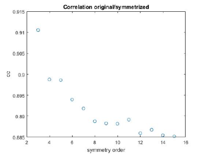
| + | Now the peaks located that at 6 and 12 are trustworthy. You can even create a new mask on the recentered average, carefully excluding intensities from the central ring structure to completely rule out any artefact. | ||
| + | |||
| + | {|style="margin: 0 auto;" | ||
| + | | [[File:FHVSymmetryAdhocMaskOverlay.png|thumb|upright|400px| Mask constructed ''ad hoc'' on the recentered average ]] | ||
| + | | [[File:FHVSymmetryAdhocMaskPlot.png |thumb|upright|400px| Symmetry merit plot using ''ad hoc'' constructed mask]] | ||
| + | |} | ||
| + | |||
| + | == Subboxing == | ||
| + | |||
| + | The ''subboxing'' technique consists in redefining the area of interest inside a previously defined average. In this example, we have use the full crowns as the subject of alignment and averaging. This has allowed us to use the whole signal carried by the full crown on each of the particles to drive the alignment robustly. This approach, however, will not allow us to identify heterogeneity and flexibility inside the individual crowns. Additionally, the possible hetereogeneity inside the crown will decrease the quality of the alignment when the crown is treated as a whole. | ||
| + | |||
| + | With the ''subboxing'' technique, we can use our previous results to setup an approach that centers the alignment on the individual teeth. Each one the particles in our new data set will be a ''subbox'' (a tooth) extracted from the previos ''box'' (the crown) using the alignment parametes for the full boxes gained by the projects that we have ran so far. | ||
| + | |||
| + | === Defining a subboxed subunit === | ||
| + | |||
| + | First, we need to define the location that we want to subbox. We use <tt>mapview</tt> | ||
| + | |||
| + | <tt>dpkdev.legacy.dynamo_mapview('localized:a') </tt> | ||
| + | |||
| + | to show the last average in the project <tt>localized</tt> | ||
| + | |||
| + | [[File:FhvSubboxSelectZ.png|thumb|center|500px| Selecting the center of the tooth subunit with <tt>mapview</tt>]] | ||
| + | |||
| + | You probably want to explore several views in mapviews (''x'/'y' and 'z') to make sure you (roughtly) hit the center of the subunit of interest. Guiding yourself only for a view on ''z'' can be misleading. | ||
| + | |||
| + | [[File:FhvSubboxSelectY.png|thumb|center|500px| Selecting the center of the tooth subunit with <tt>mapview</tt> on the ''y'' view]]. | ||
| + | |||
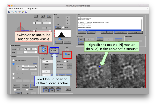
| + | As we are in this browser, we can check the size of the subunit that we want to ''subbox'', using the two markers C and N. This will be useful later when we want to actually crop physical particles using <tt>dtcrop</tt>, when we will be required to input a sidelength for the subboxed data folder. | ||
| + | |||
| + | [[File:FhvSubboxSelectDistance.png|thumb|center|500px| Measuring distances in mapview]]. | ||
| + | |||
| + | We define a variable to contain the position that we read in mapview for the blue (North) anchor. | ||
| + | <tt>rSubunitFromCenter = [88,80,53 ] - [64,64,64]; </tt> | ||
| + | We subtract the half sidelength of the full box, because the next command will need the position of the asymmetrical unit expressed in relation to center of the box. | ||
| + | |||
| + | === Creating a subboxing table === | ||
| + | |||
| + | We extract the last refined table: | ||
| + | <tt>ddb localized:rt -r t</tt> | ||
| + | |||
| + | and define positions related by C12 symmetry along the axis | ||
| + | <tt>ts = dynamo_subboxing_table(t,rSubunitFromCenter,'sym','c12');</tt> | ||
| + | |||
| + | The new subboxed table <tt>ts</tt> will have 12 times as many rows as the original one. The system of reference on each particle will point ''z'' in the direction of its original box, but the ''x'' and ''y'' orientations of each tooth will be symmetrically related in the same crown. We can depict this geometrical relationship by plotting a sketch of all the particles in the table: | ||
| + | |||
| + | <tt>figure;dtplot(ts,'m','sketch','sketch_length',100,'sm',30);view(-151,12);axis equal;</tt> | ||
| + | |||
| + | [[File:FhvSubboxSketch.png|thumb|center|500px| Sketch of orientations of the new subboxed table <tt>ts</tt>]]. | ||
| + | |||
| + | === Creating a subboxed data folder === | ||
| + | |||
| + | Now we have all we need to go back to the original tomogram and crop the subboxed particles into a new data folder using the sidelength that we checked with <tt>mapview</tt>: | ||
| + | |||
| + | <tt>dtcrop('crop.rec',ts,'subboxData',32);</tt> | ||
| + | |||
| + | We can run our typical sanity check to ensure that everything ran correctly | ||
| + | |||
| + | <tt>osb = daverage('subboxData','t',ts,'fc',1);</tt> | ||
| + | |||
| + | To visualize it you can write: | ||
| + | |||
| + | <tt>dview(osb.average);</tt> | ||
| + | |||
| + | [[File:FhvSubboxAverage.png|thumb|center|700px| Density map of the average of subboxed teeth]]. | ||
| + | |||
| + | As it looks like we expected, we just write it into a file, which we will use to define a new project. | ||
| + | |||
| + | <tt>dwrite(osb.average,'subboxRaw.em');</tt> | ||
| + | |||
| + | === Defining masks === | ||
| + | |||
| + | There are some tools to quickly format masks for project. If we want to check a reasonable radius for our mask, we can use the <tt>dsphere</tt> command and overlay the created mask on the template | ||
| + | <nowiki>cs = dynamo_sphere(10,32); | ||
| + | figure;dslices(osb.average,'y','ov',cs,'ovas','mask'); | ||
| + | figure;dslices(osb.average,'ov',cs,'ovas','mask'); </nowiki> | ||
| + | |||
| + | [[File:FhvSubboxOverlay.png|thumb|center|700px| Testing the radius of created masks by overlay on template]]. | ||
| + | In fact, this mask is probably too risky: we need a minimum of signal to drive the alignment | ||
| + | |||
| + | <tt>dwrite(cs,'maskTooth32.em');</tt> | ||
| + | |||
| + | === Subboxing project === | ||
| + | |||
| + | We create the project through: | ||
| + | <tt>dcp.new('subboxBig','d','subboxData','template','subboxRaw.em','masks','default','t','subboxData/crop.tbl','show',0);</tt> | ||
| + | |||
| + | In this case, we use <tt>'show' 0</tt> would suppress the [[dcm]] GUI. We use typically this option when we want to enter project parameters through the command line. This is exactly equivalent to entering parameters through the GUI. | ||
| + | |||
| + | <nowiki>dvput subboxBig mask maskTooth32.em | ||
| + | dvput subboxBig ite_r1 3 | ||
| + | dvput subboxBig cr_r1 4 | ||
| + | dvput subboxBig cs_r1 2 | ||
| + | dvput subboxBig ir_r1 4 | ||
| + | dvput subboxBig is_r1 2 | ||
| + | dvput subboxBig rf_r1 2 | ||
| + | dvput subboxBig rff_r1 2 | ||
| + | dvput subboxBig dim_r1 32 | ||
| + | dvput subboxBig lim_r1 [4,4,4] | ||
| + | dvput subboxBig limm_r1 1 </nowiki> | ||
| + | |||
| + | A list of the names of the parameters can be displayed through the command <tt>dvhelp</tt>. The computing environment is set using the <tt>destination</tt> parameter, shortnamed <tt>dst</tt>. To run it in matlab use: | ||
| + | |||
| + | <tt> dvput -dst matlab_parfor</tt> | ||
| + | |||
| + | For standalone running, use: | ||
| + | |||
| + | <tt> dvput -dst standalone</tt> | ||
| + | |||
| + | After running the project, we can check the effect of the independent refinement of the "tooth" units: | ||
| + | <tt>dpkdev.legacy.dynamo_mapview('subboxBig:a:ite=[0,3]')</tt> | ||
| + | |||
| + | [[File:FhvSubboxRefimentMapview.png|thumb|center|800px| Slice-to-slice comparison of initial template and final average of the subboxing project]]. | ||
| + | |||
| + | or send the average to Chimera through: | ||
| + | |||
| + | <tt>ddb subboxBig:a -c </tt> | ||
| + | |||
| + | [[File:FhvSubboxRefimentChimera.png|thumb|center|600px| Density map of the average of subboxed teeth after refinement]]. | ||
| + | |||
| + | == Visualization == | ||
| + | |||
| + | You can continue working on this data in the [[Walkthrough on creation of 3d scenes]], where you will learn to depict tomgraphic slices, place templates in table positions, and depict graphical elements representing model geometries. | ||
Latest revision as of 17:41, 3 September 2021
This walkthrough uses a small size example based on a real tomogram to cover several tasks.
Contents
- 1 The example data set
- 2 Downloading
- 3 Cataloguing the tomogram
- 4 Annotation of particle positions
- 5 Cropping particles
- 6 Project to find membrane orientations
- 7 Aligning the axis of symmetry
- 8 Using the membrane to impart an orientation
- 9 Project for rotational alignment
- 10 Project with rotational randomization
- 11 Project for localized alignment
- 12 Subboxing
- 13 Visualization
The example data set
The data is a fraction of a tomogram. The full tomogram was used in "Cryo-electron tomography reveals novel features of a viral RNA replication compartment." (Ertel et al.), and represents several FHV viruses docked in the outer membrane of a mitochondrion.
Downloading
During the Dynamo workshop you will find the needed tilt series in your data folder. Outside the workshop, you can download all the files related to this example with the command:
dpkhelp.wiki.downloadExample('fhv');
If it fails under Matlab or the Dynamo command line, you can try to directly use the linux order
wget https://wiki.dynamo.biozentrum.unibas.ch/w/doc/data/fhv/crop.rec
or
curl -O https://wiki.dynamo.biozentrum.unibas.ch/w/doc/data/fhv/crop.rec
under MacOS. This should have created the file called crop.rec in your current directory.
Size check of a file
You're probably curious to see what's inside, so that let's write first:
dfile crop.rec
to let Dynamo check the dimensions of the file. The header of a .rec file is readed as a regular mrc, yielding:
 filetype: volume
 size: 1285 x 956 x 786
So, it's a tomogram.
Lightweight visualization
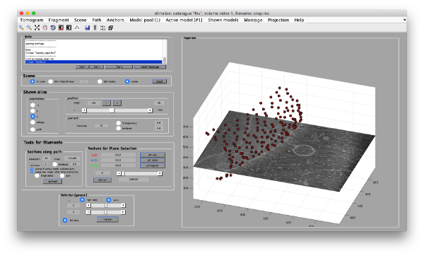
We can inspect quickly its contents with dtmshow
dtmshow -otf crop.rec
Hereby, the flag -otf means "on the fly", telling dtmshow to not preload the full tomogram, but to access in disk the individual slices that are needed when inspecting a particular area.
Go up and down. We want to select the locations were the vesicles intersect the mitochondrion membrane and average them together. For this, we need to catalogue the tomogram, so that our annotations are stored with a clear relationship with the tomogram.
Cataloguing the tomogram
We can create catalogues just to contain a single tomogram. They are useful to keep track of all annotations, and of the typical transforms (binning, cropping of fractions) that we usually perform on a larged size tomogram of interest. In this case, we can create the catalogue directly from the command line:
dcm -create fhv
where dcm is the short form of dynamo_catalogue_manager and fhv is just an arbitrary name. The just created catalogue is empty, and we can add our tomogram with:
dcm -c fhv -at crop.rec
We can check that the tomogram is in the catalogue by asking Dynamo to show the contents of the catalogue
dcm -c fhv -l tomograms
or
dcm -c fhv -l t
The flag -l asks Dynamo to list items of a given category of catalogue contents, in this case tomograms
Prebinning the tomograms
We typically want to prebin the tomogram, i.e., have a version of |smaller size that is known to the catalogue. This version will be useful in some operations that require a full tomogram in memory, an operation that can consume much memory and need a long time. In this example, this would not be necessary: a tomogram with a sidelength on x and y of ~1000 pixels shouldn't pose any visualization problem. We do it anyway for the exercise with the command:
dynamo_catalogue_bin('fhv', 1, 'zchunk', 300);
where the parameter zchunk represents the maximum number of z slices that are kept simultaneously in the memory during the binning process. This parameter might be important for larger size tomograms.
Operation with GUI
These steps could have been performed thorough the dcm GUI
Annotation of particle positions
Now we can open the tomogram through the catalogue:
dtmslice crop.rec -c fhv -prebinned 1
Probably you don't like the initial contrast, change it with the button in the toolbar.
- left click and drag the slice with your mouse to move it up and down
- this can also be achieved with the controls on the left hand side
- ctrl + left click and drag will change your viewpoint of the 3d scene
- shift + left click and drag will move the center of rotation
- ctrl + mouse wheel up/down will zoom in or out of the scene
Other axiliary tools are the keys x,y,z to change the slice orientation, the number of projected slices (called "thickness" in the GUI controls), the transparency of the slice.
You can reset the scene at any time by hitting the reset button.
You can save slices for viewing later with the s key.
Creation of models to contain annotations
In this example we just want to manually pick some particles. This can be done creating a general or box model, which will reside in memory till we save it into the catalogue.
After creating the model, it will be only model currently active in the dtmslice scene. You can add new points pressing on [c]. The idea is to mark on the positions where you see the "neck" of a vesicle (what we called "crowns") in contact with the outer mitochondrial membrane.
The last marked point can be deleted by pressing [delete]. An arbitrary point can be deleted by clicking on it with the auxiliary mouse button. This will open a menu that includes the option of deleting the point (through Ctrl+X in Linux or Cmmd+X in Mac).
At this stage you probably want to change the transparence of the depicted slice, so that you can control which objects have been already clicked below the depicted slide.
.
When you are done, remember to save the model, using the menu options on active model or simply clicking on the disk icon in tomoslice.
Cropping particles
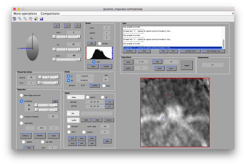
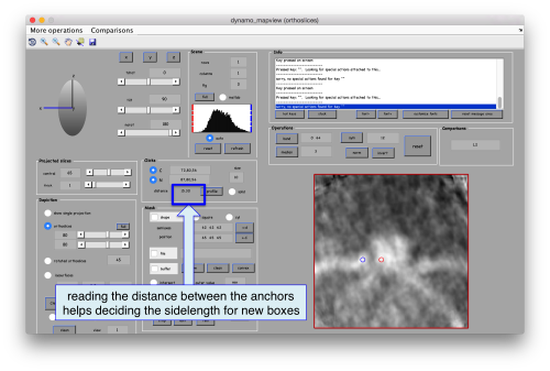
Now we want to use the positions that we have marked to extract the subtomograms and format them as a data folder. The first thing we need is an estimation of the sidelength in pixels of each of the subtomograms. In dtmslice We can use the keys [1] and [2] to define two anchor points that appear as rombohedra. Clicking (with the right button) onto the black dashed that links the will show on screen both coordinates and the distance between them. All distances are reported in pixels of the non-binned tomogram: even if you are using a binned version, Dynamo keeps track of it.
.
We will thus choose to create a datafolder with a cubic sidelength of 128 pixels (remember that the particles will be cropped in the unbinned tomogram). This will ensure that the crowns fit comfortably inside the physical box, even if our manual picking imposes an error of several pixels. If you were using, say, a thickness parameter of 10 pixles in dtmslice, you have to count with at least this inaccuracy in the location of the particles.
Now, we check that the catalogued tomogram contains the model that we manually picked before:
>> dcmodels fhv
Volume 1 contains 1 models in total
/Users/casdanie//fhv/tomograms/volume_1/models/mboxes.omd
In your system, instead of /Users/casdanie/ you will see the path to the folder where you created the catalogue fhv
Creating a table
We could just use the catalogue GUI to extract the particles, be it is also possible to proceed directly with the command line. We will use the dtcrop command, .which requires preparing a table with the information of the model.
m = dread('/Users/casdanie/fhv/tomograms/volume_1/models/mboxes.omd');
t = m.grepTable();
Here, you read the file into a model object (which we arbitrarily choose to call m), and then you use the grepTable method on this object to extract a variable into your workspace. We arbitrarily call it t.
Note that we can extract models directly from the output of dcmodels
dcmodels fhv -i 1 -ws o;
m = dread(o.files{1});
t = m.grepTable();
i.e., we load the answer of dcmodels for volume index -i 1 in the output variable o. Inside it, there is a field called 'files' which contains a cell array of files containing models. Then we read the first entry o.files{1}.
Whichever way you create the table variable t, it is just a matrix with a row for each particle, and a summary of the information coded inside can be created through:
>> dtinfo(t);

        size                :  22 35
        NaNs                :  0

 COLUMN
[  2  ] marked for alignment:  22
[  3  ] included in average :  22
[ 4-6 ] shifts              :  all zero
[ 7-9 ] angles              :  all zero
[  10 ] cross correlation   :  min: 0.00  max: 0.00  mean: 0.00  std: 0.00
[  13 ] Fourier sampling    :  1 (single tilt around y)
[  13 ] fsampling types     :  all of the same type
[14-15] ytilt range         :  min:120.00   max:120.00
[16-17] xtilt range         :  min:120.00   max:120.00
[  20 ] linked volumes      :  total 1 (labels: [1])
[  21 ] regions inside tomograms :  total 1 (labels: [0])
[  22 ] user-defined classes:  total 1 (labels: [0])
[  23 ] annotation types    :  total 1 (labels: [0])
[24-26] spatial locations   :  initialized: 22
[  24 ]   *  x              :  min: 645.21  max: 1001.92  mean: 799.05  std: 109.44
[  25 ]   *  y              :  min: 23.78  max: 917.51  mean: 484.07  std: 271.28
[  26 ]   *  z              :  min: 198.00  max: 563.00  mean: 415.55  std: 114.03
[  31 ] original tags       :  total 1 (labels: [0])
[  32 ] compacted particles :  total 1 (labels: [1])
[  34 ] references          :  total 1 (labels: [0])
[  35 ] subreferences       :  total 1 (labels: [0])
[  36 ] apix                :  Warning: column not available in this table
[  37 ] defocus             :  Warning: column not available in this table
Using dtcrop
The simplest syntax of dtcrop requires passing the name of the tomogram from which we want to crop (syntax varies for cropping from multiple tomograms). We know that the file is crop.rec, and we could directly insert this name in the command. But a catalogued model already contains information about its source tomogram (inside its property cvolume), so that we can always track it back. We could then define a variable tomogramFile by accessing this information inside the model variable m:
tomogramFile = m.cvolume.file();
if you get a warning at this stage, don't worry, the command still worked.
You can then launch the cropping order:
o = dtcrop(tomogramFile,t,'particlesData',128);
where you could add the mw flag to let Dynamo use several cores. In any case, for this number or particles the cropping should take some seconds. The last part of the final output into screen should look like this:
21 [read_subtomogram] Volume has size 1285 956 786
[read_subtomogram] Accessing subvolume x: 713:840; y: 339:466; z: 160:287  totalling ~ 16.0Mb
Elapsed time is 0.191014 seconds.
22
Total time invested in cropping: 7s
[table_crop] Done extracting 20 particles
             from tomogram      :"/Users/casdanie/dynamo/devmac/workplace/paris/crop.rec"
             destination folder :"particlesData"
             excluded particles : 2

 [ok] table_crop
informing you that some of the particles where excluded, as they were probably too close to the boundary of the tomogram, given the sidelength we asked for. Inside the created data folder, you will find the table particlesData/crop.tbl, which only indexes the actually cropped particles.
Creating an average
The particles can now be averaged together. They have different orientations, but in this tomogram we only have a fraction of the membrane.
oa = daverage('particlesData','t','particlesData/crop.tbl');
If you want to let Dynamo pass maps into Chimera, you have to inform Dynamo on the location of Chimera. For instance:
dchimera -setPath /usr/local/bin/
Please adapt it to the location of Chimera in your file system.
To open your average in chimera
dchimera(oa.average)
Project to find membrane orientations
We first need to create files with the average and the table that we have till now in memory:
dwrite(t,'raw.tbl');
dwrite(oa.average,'rawTemplate.em');
We can create a project directly thorugh the command line:
dcp.new('first','d','particlesData','template','rawTemplate.em','masks','default','t','particlesData/crop.tbl');
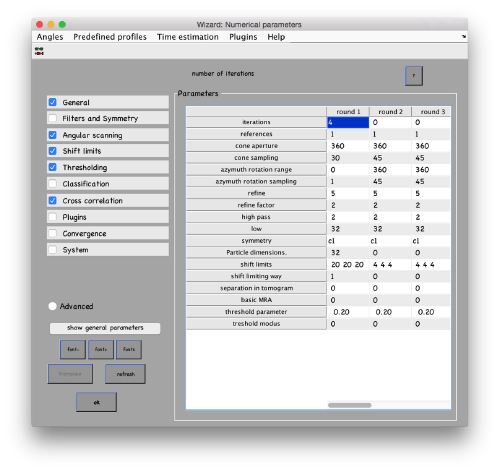
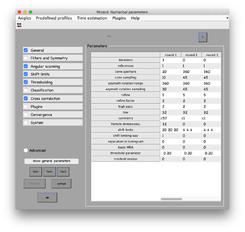
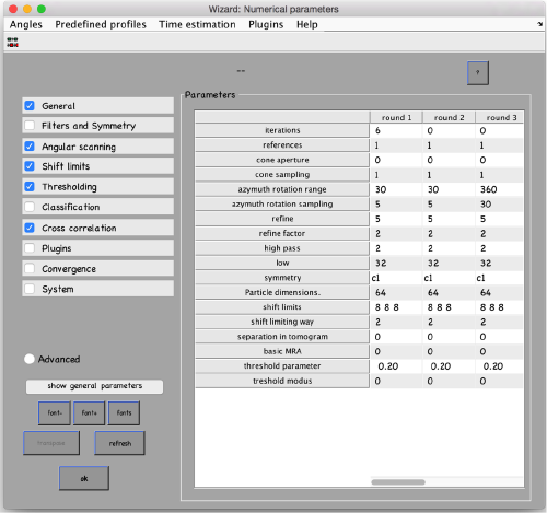
...and go directly to the panel of numerical parameters to create a project adapted for catching the general orientation of the membrane:
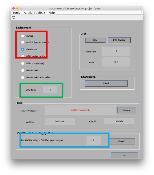
Also, remember to visit the window for execution environment, and select the appropriate settings. If you are working with Matlab, select Matlab(for one single core) or "Matlab_parfor" (if you are going to several cores). If working with the standalone, use the standalone option. In both cases, select the number of cores for alignment (green box in the picture below) and averaging (blue box) .
You can operate the project management operations from the GUI or the command line. First checking:
dvcheck first
then unfolding
dvunfold first
and finally running it by invoking the name of the execution script. If you are running in Matlab use:
first
If you are running Dynamo in standalone modus, open a new tab (or window) of the terminal, load Dynamo (but don't run Dynamo) and type:
./first.exe
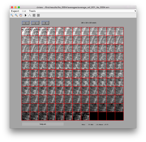
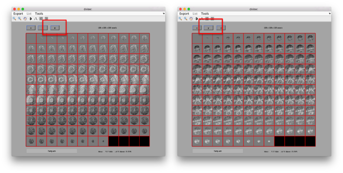
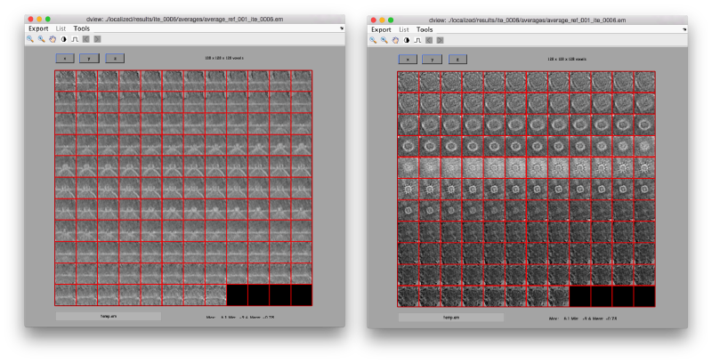
After running the project, we check the created average:
ddb first:a -v
This command asks the database (hence db) of the project first to look for the item of type average, by default accessing the last computed one. The flag -v sends the output of the database query to the depiction GUI called dview.
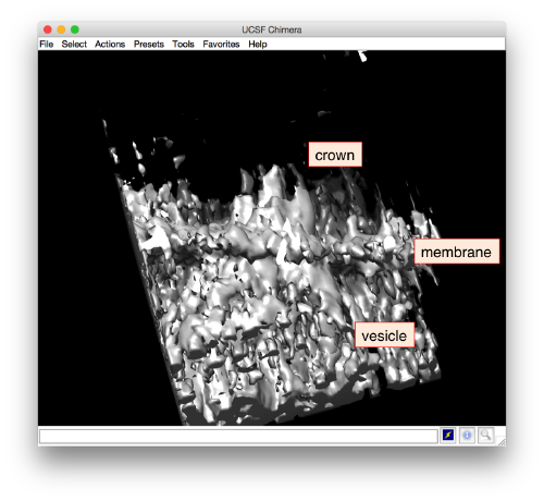
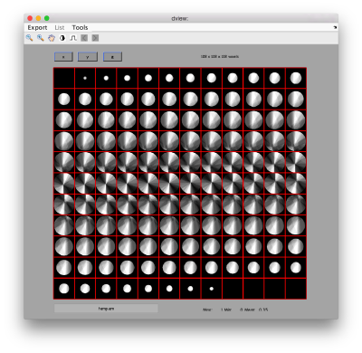
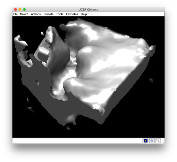
Apparently, the project finds the membranes and centers the particles correctly. If you show the volume in Chimera (by clicking in the Export>Send to Chimera option in the dview window ).
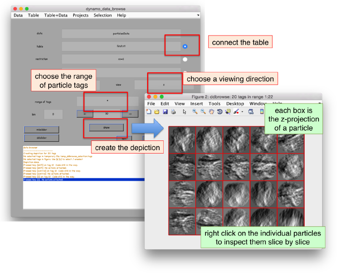
We can check the individual particles:
ddbrowse -d first:data -t first:rt
.
Aligning the axis of symmetry
We would like to bring the axis of symmetry to the zdirection. This will create an intuitive separation between the two first euler angles that represent "change of orientation of the main axis", and the third one that represents "azimuthal rotation about the new axis". We want that azimuthal rotations occur about an axis of possible symmetry, which by convention is located along z. There are several ways to achieve this. A simple one is to create a model of the membrane/crown geometry, align our average to it (with dalign), and use the alignment parameters to create a new table. With this new table and average we will be able study possible symmetries with a new project.
Creating a template aligned with z
Geometrical shapes of many types can be created with dmask,dsphere,dcylinder,dshell and dtube, and combined with dynamo_mask_combine. However, there are also some available utilities to create templates representing frequently occurring membraneous geometries:
mr = dpktomo.examples.motiveTypes.MembraneWithRod();
mr.sidelength = 128;
mr.rodRadius = 20; mr.rodShift = [0,0,10]; mr.rodHeight= 20;
mr.getMask();
template  = mr.mask;
Note that you can check the list of properties inside the object mr just by typing it without the semicolon and pressing [Return]
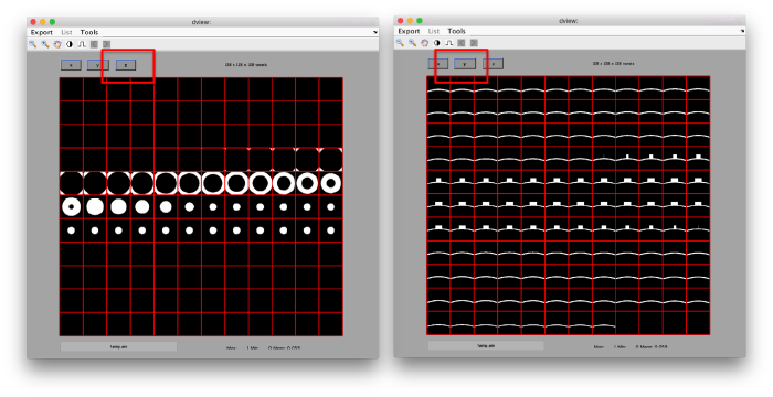
We can check the result with:
mr.viewMask();
Aligning the previous average along z
The mask is white on black by definition. The tomogram data in this case represents bright protein on dark background, so that in this case we want to align the previously computed average to the mask of the mr object.
The alignment does not need to scan azimuthal rotations, so that our 'inplane_range' will be 0. The 'cone_range' will be the full sphere, and we take and spacing of 30 degrees. As we are looking for coarse orientations, we can bin the two volumes twice (yielding volumes with a sidelength of 32 pixels). We will also "nail" the new center to the physical center of the box (parameter limm set to 1 below).
Now we read the average computed by the project first into a workspace variable which we arbitrarily call previousAverage
ddb first:a -r previousAverage;
Here, the volume previousAverage will be treated as a "particle" to be aligned onto a template, which in this case is the volume contained in mr.mask.
sal = dalign(previousAverage,mr.mask,'cr',360,'cs',30,'ir',0,'dim',32,'limm',1,'lim',[10,10,10]);
The flags are the same parameters that would be used in an alignment project. You can check the shorthands with dvhelp.
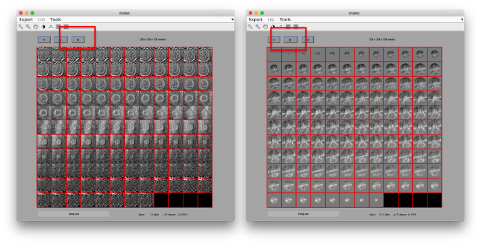
The output result sal contains many fields. We can, for instance directly visualize how the previous average looks like when transformed through the results of this dalign operation. For this, use the field aligned_particle in the output sal:
dview(sal.aligned_particle);
Applying the z-alignment to the table
We don't want just to get a z-oriented average: we also want to convert the table yield by the first project into a table that, when applied onto the original data, produces a correct, z-aligned average. For this, we use the alignment parameters coded inside the output sal (as field .Tp) and apply them onto the table.
ddb first:rt -r tf
The variable tf contains now the original table, which is now rotated and shifted according with the rigid body transform Tp inside sal
tr = dynamo_table_rigid(tf,sal.Tp);
now the rectified table tr should contain the metadata that makes the particles "point upward". We use now the typical sanity check to assess that a table behave as expected: we apply it to the particles in its paired data folder and check the average:
oz = daverage('first:data','t',tr,'fc',1);
whose results can be checked by:
dview(oz);
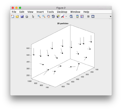
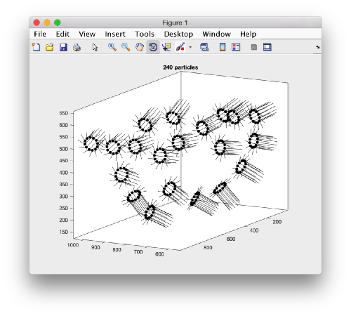
We can visualize this operation by plotting a sketch with the orientation of the particles. We first show the results for the table computed in the project first
figure;
dtplot('first:rt','m','sketch','sketch_length',100,'sm',30);
view(-230,30);axis equal;
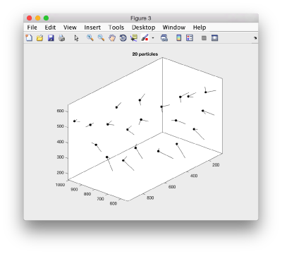
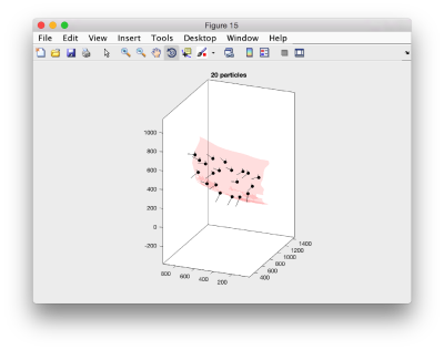
Here, the 'z' orientation computed for each particle is represented by the longest semiaxis. Note that with the original definition of the template, the 'z' points -approximately- along the direction of the 'z' in the tomogram. If we depict the same plot with the table we just computed:
figure;
dtplot(tr,'m','sketch','sketch_length',100,'sm',30);
view(-230,30);axis equal;
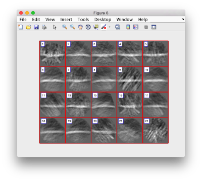
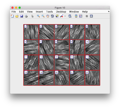
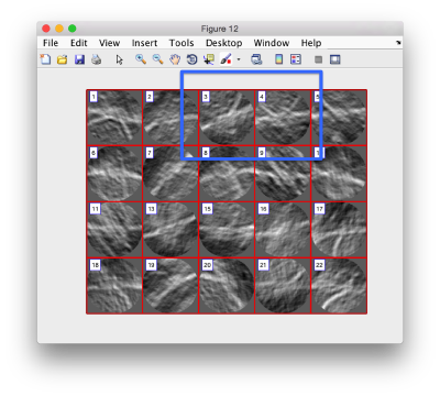
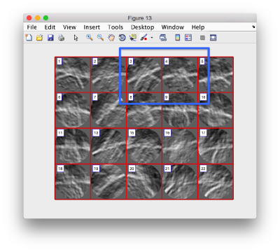
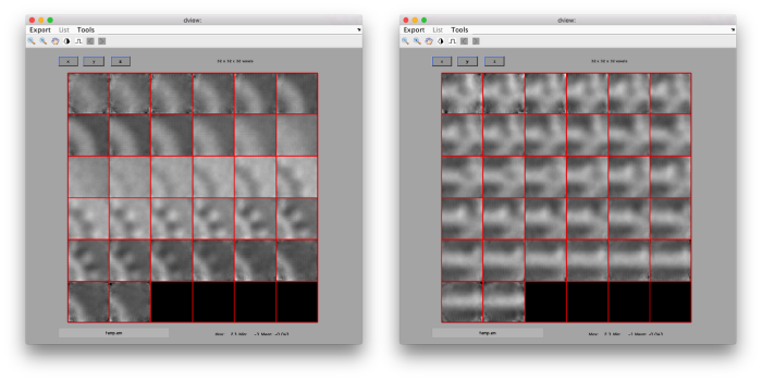
we see that now the 'z' axis in each particle is pointing orthogonally(-ish) to the membrane. A different quick check would be to show the projections of the particles along y. Instead of using the GUI ddbrowse, we can create this depiction with a single command:
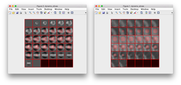
figure;dslices('particlesData','t',tr,'projy','*','align',1,'labels','on');
Lets look at the z-projection. In this case we project only the central slices around the crown and the aperture in the viral vesicle, chosing thus slices 60 to 70. if project the full particle, we won't distinguish any features.
figure;dslices('particlesData','t',tr,'projz',60:80,'align',1,'labels','on');
The depiction clearly shows the missing wedge of the particles. Incidentally, it also shows that averaging all the particles should produce an average that covers all the orientaions in the Fourier space.
Using the membrane to impart an orientation
This section describes an alternative method to compute:
- a rough orientation of the particles, and
- a rough first template
In this section we will use the membrane of the mithocondrion to assign a roughly orientation to each of the points in the table. This orientation will be defined by the normal of the closest point in the membrane. The membrane will be defined as a a triangulation, to be constructed based on a set of manually picked points.
Pick membrane points
We open our tomogram in dtmslice
dtmslice @{fhv}1 -prebin 1
or, if you are working with the standalone version, please prepend a "\" symbol:
\dtmslice @{fhv}1 -prebin 1
In this variant of the syntax of dtmslice, the string @{fhv}1 just means "tomogram number 1 inside catalogue fhv. On the opened scene, we will use a montage to manually click on a set of membrane points.
Note! (08/06/21) - the montage viewer was recently updated and no longer provides the ability to easily add points, please define your surface model on sequential z-slices in dtmslice directly by annotating points every 20 or so slices.
By default, this montage represents slices taken orthogonally to z every 20 pixels of the unbinned tomogram. This can be changed in the settings before opening the montage GUI. Now, we can create a model of type Surface, which we will use to store a set of points in the membrane to be picked manually (or semiautomatically). To do this, go to Model pool> Create new model in pool (choose type) > surface
You need to click on the point switcher (the control in the toolbar with a c and an i) to allow entering points. The basic controls are:
- Mouse click to enter a point.
- d to delete a point.
- i to insert a point.
Use the >> button in the bottom of the GUI to go to next set of orthoslices.
Note that the points that you click in the Montage GUI are assigned to a model in the pool, and as such, they appear automatically in the dtmslice GUI
You also need shift + C in order to place a center inside the mithocondrion. This point is just used to tell Dynamo what is the inside and what is the outside face of the surface that we are building.
Automatic detection
Once you have clicked points on a level, you can try and check if the automatic tracker can locate them in the next one. To do so, activate the next slice (i.e., secondary click it, so that its frame becomes red), and press o. You can edit the points with d to delete the closest point, m to move the closest point to the position currently under the cursor, or l to delete all the points detected in the slice... in such a case, you probably want to check the tracking parameters before using o again!
Create a surface
Now, we want to convert the points that we have introduced into a triangulation. This is a part of the workflow used to crop particles from membrane models, so we open the workflow GUI for this model in the Active Model menu tab.
We can first check the points currently contained in the model, by auxiliary clicking on the first viewing option and choosing the User points option. They will be depicted in a graphic window which will update with the new graphical elements that we depict there.
We first need to create a spline interpolation on each of the levels of our point cloud.
Now we define a triangulation on this control points.
Which can be subdivided to get a smoother appearance, and also a more accurate representation of the geometry.
Then, we can change the name of the model for clarity, and then save it into the catalogue (with the disk icon in tmslice or the Save into catalogue options under the Active model menu)
Use a surface to impart orientation
We bring the model into our workspace. We search for it in the catalogue:
dcmodels fhv -nc mySurface -ws output
which will prompt the response
Volume 1. Matching models: 1 (total: 1)
/Users/casdanie/dynamo/examples/fhvParis/fhv/tomograms/volume_1/models/mySurface.omd
now, we can read the model file into our memory space to operate with it:
m = dread(output.files{1});
Now the model m is in our space of memory and can be used to impart an orientation to the points in our table.
tOrientedBySurface = dpktbl.triangulation.fillTable(m,'raw.tbl');
In this table, orientations are orthogonal to the membrane (or more precisely, orthogonal to the closest triangle in the mesh that represents the membrane)
figure;dslices('particlesData','t', tOrientedBySurface,'projy','c20','align',1,'labels','on');
tConsistent = dynamo_table_flip_normals(tOrientedBySurface,'center',m.center)
We can check the effect of this table on the particles through:
figure;dslices('particlesData','t', tConsistent,'projy','c20','align',1,'labels','on');
To get a better graphical impression, we can depict our surface (contained in the model m) with:
m.ezplot
and choose the Surfaceoption
Then, we just plot the positions of the particles on the same graphical figure:
dtplot(tConsistent,'m','sketch','sketch_length',100,'sm',30);
Management of the missing wedge
When we create a table considering only the orientations of the points with relation to a membrane, there is no particular preference for rotations of the particles about the normal direction (i.e., azimuthal directions). The narot angle in this table is initialized to zero
Thus, take into account that an average created on these particles will have a strong missing wedge, especially in our case, where we have a preferential direction. This can be checked by averaging the particles against this table:
oa=daverage('particlesData','t', tConsistent,'fc',1);
Here, we ask ('fc',1) to run a Fourier compensation step, so that we can check in the output oa the property fweight, which contains the number of times a Fourier component is represented in the average. Bright values mean that the Fourier component is present in many particles (yielding thus an average of better quality for the involved frequencies).
dview(oa.fweight);
We can atenuate this effect by randomizing the rotational angle:
tConsistentRandomized = dynamo_table_randomize_azimuth( tConsistent);
and averaging again.
oaRandomized=daverage('particlesData','t', tConsistentRandomized,'fc',1);
Now, the fweight map doesn't show such a strongly preferential orientation:
dview(oaRandomized.fweight);
The effect in direct space can be shown by depicting both averages (with and without randomization side to side)
dpkdev.legacy.dynamo_mapview({oa.average,oaRandomized.average});
Project for rotational alignment
We have now a template and a coherently defined metadata (i.e. table) that align the particles coarsely along the right direction. We write them into disk: Insert non-formatted text here If you did not create a membrane model, use the results of the alignment project:
dwrite(tr,'zOriented.tbl');
dwrite(oz.average,'zOriented.em');
If you did create a membrane model, used the corresponding table and average:
dwrite(tConsistentRandomized,'zOriented.tbl');
dwrite(oaRandomized.average,'zOriented.em');
and create a project with these files. Note that the data folder remains unchanged.
dcp.new('zOriented','d','particlesData','template','zOriented.em','masks','default','t','zOriented.tbl');
In this project, we will ask for a symmetrization 'c57'.. this is just to simulate fully rotational symmetry. We are not assuming that this symmetry is physical: we just want to force any possible symmetry axis in the data along the z axis. We also keep binning twice the particles, in order to get the computation times short.
The result shown an incipient formation of the crown... however, the presence of suspicious striations in a preferential direction might be an indication of the effect of the missing wedge.
Project with rotational randomization
We can create a template that does not have a prefererential orintation, by just randomizing the azimuthal rotations in our table, We extract the last refined table into the variable tns
ddb zOriented:rt -r tns
and impose a perturbation that keeps all other parameters constant but randomly rotates the particles around their axis
tr = dynamo_table_perturbation(tns,'pshift',0,'paxis',0,'pnarot',360);
We can use this table to average again the particles and check the average.
oar = daverage('particlesData','t',tr,'fc',1);
dview(oar)
Now, we can write these files in disk and create a project:
dwrite(oar.average,'randomizedAverage.em');
dwrite(tr,'randomized.tbl');
dcp.new('zRandomized','d','particlesData','template','randomizedAverage.em','masks','default','t','randomized.tbl');
After running this projects, the presence of a crown-like is very, very faintly hinted in mapview:
dpkdev.legacy.dynamo_mapview('zRandomized:a')
and barely identifialble in Chimera:
Project for localized alignment
We don't see clearly what is happening on the area of interest... On one hand we know that we are using a very reduced number of particles ( which on top of it are too similarly oriented). But there is still some room to improve in the approach: we can focus the refinement in the area of interest.
Creating a tight mask
We want to create a mask that encloses the area of interest. To do this, we open the average in dmapview:
dpkdev.legacy.dynamo_mapview('zRandomized:a')
We tune the browser for viewing along y, and we select one of the central slices. We can use a thickness of several pixels to have a better view.
Then, we select the area that we want to use as seed in this plane to create a revolution solid. We press on [shift] + [s] on the selected slide, letting a new window pop up. In this window, you handdraw an area on the XZ plane (main click to start drawing, auxiliary click to stop). Dynamo will rotate the region about the z axis, creating a revolution solid into the file temp_drawn_revolution_mask.em
We have to change the default name given by Dynamo to a relevant one:
!mv temp_drawn_revolution_mask.em teethMask.em
and now continue the previous project by transferring the results of zRandomized to a fresh project (lets call it localized)
dynamo_vpr_branch zRandomized localized -b 1 -noise 0
where we insert the tight mask teethMask.em that we just created as alignment mask of the project. Note that we do not want impose any symmetry in our parameters:
Let's inspect the output in dview
There are different things that we like in this average
- The localized masking worked well, producing a clearer insight into the region of relevance
- Although we are using signal only inside the mask, the material outside of the mask does 'not become smeared. This is clear mark that the alignment is real and non artifactual. That's an important point to check when we use small masks.
- The symmetry in the area becomes apparent on the bare eye. They can be distinguished clearly with mapview and even in Chimera.
Testing the symmetry
We can check for different symmetry operators to confirm the presence of symmetry.
Basic command
The basic command for this task is dynamo_symmetry_scan. In its fundamental syntax, you need to state the type of symmetry operator to be tested, and a set of operator.
stm = dynamo_symmetry_scan('localized:a','c','order',3:15,'type','pearson','nfig',3);
With a more localized mask:
slm = dynamo_symmetry_scan('localized:a','c','order',3:15,'type','pearson','mask','teethMask.em','nfig',4);
Interpretation of results
If you got the results above, you might have jumped to the conclusion that they already constitute an objective hint at a real C12 symmetry. This is, however, not true. The fact is that, with a slightly different picking of particles, you could have obtained the profiles in these pictures:
These images represent the result of the two symmetry-exploring commands described above obtained by a different user. . Surprisingly, they point at possible symmetry orders of 11 and 13. So, what is going on here? How is it possible that two different users that operate exactly the same walkthrough get contradictory symmetry estimations? The reason is that different users will pick manually slightly different particle centers, and this have a direct impact on the symmetry estimation. In short, the problem is that the density map localized:a is not garanteed to have its possible symmetry axis located along the center of the box, and this misleads dynamo_symmetry_scan. This can bechecked by opening the average in mapview and overlaying the file 'teethMask.em' on it.
In this non-centered density map, any symmetry determination can only be an artifact. To solve this, we create a centered version:
ddb zOriented:a -r zo % extract average of zOriented as the ws variable zo
ddb localized:a –r localizedAverage % extract average of localized as the ws variable localized Average
sal = dalign(localizedAverage,zo,'cr',0,'cs',30,'ir',0,'dim',64,'limm',1,'lim',[20,20,20]); % aligns localizedAverage against zo (like that localizedAverage is centered)
centerLocalized = sal.aligned_particle;
dview(centerLocalized);
We can scan again the symmetry operators on the recentered volume.
slmCentered = dynamo_symmetry_scan(centerLocalized,'c','order',3:15,'type','pearson','mask','teethMask.em','nfig',4);
Now the peaks located that at 6 and 12 are trustworthy. You can even create a new mask on the recentered average, carefully excluding intensities from the central ring structure to completely rule out any artefact.
Subboxing
The subboxing technique consists in redefining the area of interest inside a previously defined average. In this example, we have use the full crowns as the subject of alignment and averaging. This has allowed us to use the whole signal carried by the full crown on each of the particles to drive the alignment robustly. This approach, however, will not allow us to identify heterogeneity and flexibility inside the individual crowns. Additionally, the possible hetereogeneity inside the crown will decrease the quality of the alignment when the crown is treated as a whole.
With the subboxing technique, we can use our previous results to setup an approach that centers the alignment on the individual teeth. Each one the particles in our new data set will be a subbox (a tooth) extracted from the previos box (the crown) using the alignment parametes for the full boxes gained by the projects that we have ran so far.
Defining a subboxed subunit
First, we need to define the location that we want to subbox. We use mapview
dpkdev.legacy.dynamo_mapview('localized:a')
to show the last average in the project localized
You probably want to explore several views in mapviews (x'/'y' and 'z') to make sure you (roughtly) hit the center of the subunit of interest. Guiding yourself only for a view on z can be misleading.
.
As we are in this browser, we can check the size of the subunit that we want to subbox, using the two markers C and N. This will be useful later when we want to actually crop physical particles using dtcrop, when we will be required to input a sidelength for the subboxed data folder.
.
We define a variable to contain the position that we read in mapview for the blue (North) anchor.
rSubunitFromCenter = [88,80,53 ] - [64,64,64];
We subtract the half sidelength of the full box, because the next command will need the position of the asymmetrical unit expressed in relation to center of the box.
Creating a subboxing table
We extract the last refined table:
ddb localized:rt -r t
and define positions related by C12 symmetry along the axis
ts = dynamo_subboxing_table(t,rSubunitFromCenter,'sym','c12');
The new subboxed table ts will have 12 times as many rows as the original one. The system of reference on each particle will point z in the direction of its original box, but the x and y orientations of each tooth will be symmetrically related in the same crown. We can depict this geometrical relationship by plotting a sketch of all the particles in the table:
figure;dtplot(ts,'m','sketch','sketch_length',100,'sm',30);view(-151,12);axis equal;
.
Creating a subboxed data folder
Now we have all we need to go back to the original tomogram and crop the subboxed particles into a new data folder using the sidelength that we checked with mapview:
dtcrop('crop.rec',ts,'subboxData',32);
We can run our typical sanity check to ensure that everything ran correctly
osb = daverage('subboxData','t',ts,'fc',1);
To visualize it you can write:
dview(osb.average);
.
As it looks like we expected, we just write it into a file, which we will use to define a new project.
dwrite(osb.average,'subboxRaw.em');
Defining masks
There are some tools to quickly format masks for project. If we want to check a reasonable radius for our mask, we can use the dsphere command and overlay the created mask on the template
cs = dynamo_sphere(10,32);
figure;dslices(osb.average,'y','ov',cs,'ovas','mask');
figure;dslices(osb.average,'ov',cs,'ovas','mask');
.
In fact, this mask is probably too risky: we need a minimum of signal to drive the alignment
dwrite(cs,'maskTooth32.em');
Subboxing project
We create the project through:
dcp.new('subboxBig','d','subboxData','template','subboxRaw.em','masks','default','t','subboxData/crop.tbl','show',0);
In this case, we use 'show' 0 would suppress the dcm GUI. We use typically this option when we want to enter project parameters through the command line. This is exactly equivalent to entering parameters through the GUI.
dvput subboxBig mask maskTooth32.em
dvput subboxBig ite_r1 3
dvput subboxBig cr_r1 4
dvput subboxBig cs_r1 2
dvput subboxBig ir_r1 4
dvput subboxBig is_r1 2
dvput subboxBig rf_r1 2
dvput subboxBig rff_r1 2
dvput subboxBig dim_r1 32
dvput subboxBig lim_r1 [4,4,4]
dvput subboxBig limm_r1 1
A list of the names of the parameters can be displayed through the command dvhelp. The computing environment is set using the destination parameter, shortnamed dst. To run it in matlab use:
dvput -dst matlab_parfor
For standalone running, use:
dvput -dst standalone
After running the project, we can check the effect of the independent refinement of the "tooth" units:
dpkdev.legacy.dynamo_mapview('subboxBig:a:ite=[0,3]')
.
or send the average to Chimera through:
ddb subboxBig:a -c
.
Visualization
You can continue working on this data in the Walkthrough on creation of 3d scenes, where you will learn to depict tomgraphic slices, place templates in table positions, and depict graphical elements representing model geometries.
