Difference between revisions of "Indicating the missing wedge"
(Created page with "''Dynamo'' needs to know the missing wedge of the particles. == In the table == The missing wedge of each particle is expressed in columns 13 to 19 of a table (remember that...") |
AlisterBurt (talk | contribs) |
||
| (3 intermediate revisions by one other user not shown) | |||
| Line 3: | Line 3: | ||
== In the table == | == In the table == | ||
The missing wedge of each particle is expressed in columns 13 to 19 of a table (remember that a row represents a single particle). | The missing wedge of each particle is expressed in columns 13 to 19 of a table (remember that a row represents a single particle). | ||
| − | In this system, column 13 represents the [[Table_column_convention#col 13: ftype (type of fourier sampling) | type of missing wedge]] and the rest of columns are used to express the tilt range in y,x, and z. | + | In this system, column 13 represents the [[Table_column_convention#col 13: ftype (type of fourier sampling) | type of missing wedge]] and the rest of columns are used to express the tilt range in y, x, and z. Only the relevants columns for each case are taken into account. |
== In the catalogue == | == In the catalogue == | ||
| Line 9: | Line 9: | ||
==Custom missing wedge== | ==Custom missing wedge== | ||
| + | Built-in fourier types represent solid wedges. You can choose to use a customized missing "wedge" for each particle by storing them as separate files in the same [[Data folder#Fourier Mask on particles| data folder]] where you have your particles (each Fourier mask is represented by a <tt>pfmask_XXXX.em</tt> file). In this case, you need to choose <tt>ftype</tt> 5 in the table. | ||
| + | |||
| + | ==Tilt range== | ||
| + | |||
| + | What is exactly the tilt range that you need to input? For solid wedges with a symmetric extent (i.e., -60 to 60) it is rather trivial. For the asymmetric case, it might be more difficult: it will depend on the reconstruction program you used, and how it handled the alignment. Lets assume a <tt>ftype</tt> 1 (i.e., column 13 of table will be one). In this geometry, electrons come from the direction z, and the sampled rotated around the 'y' direction in a range of theta angles whose extremal values will be indicated in columns 14 and 15. | ||
| + | |||
| + | In principle, you could think that if your tilt series goes from -45 to 60” you should write <tt>45</tt> in column 14 and 60 in column 15. But it is a little more complicated than that. Depending on how you have chosen the orientation of the tilt axis when aligning the raw micrographs, you might need to actually write the option combination [-60,45]. | ||
| + | |||
| + | In order to be certain about ''Dynamo'' parametrized the missing wedges, you can just create the two versions: | ||
| + | |||
| + | <nowiki>figure;f = dfmask(64,[-45,60]);dslices(f,'x|y|z','j','*');title('-45:60');shg | ||
| + | figure;f = dfmask(64,[-60,45]);dslices(f,'x|y|z','j','*');title('-60:45');shg </nowiki> | ||
| + | |||
| + | and check the results: | ||
| + | |||
| + | {|style="margin: 0 auto;" | ||
| + | | [[File:MissingWedgeminus45To60.png|thumb|upright|400px| missing wedge of type 1 with ''y'' range -45:60]] | ||
| + | | [[File:MissingWedgeminus60To45.png|thumb|upright|400px| missing wedge of type 1 with ''y'' range -60:45l]] | ||
| + | |} | ||
| + | |||
| + | Then you compare it to how a particle of your data set looks like. If <tt>myParticle</tt> is a random particle out of your tomogram you can write: | ||
| + | |||
| + | <tt>dynamo_wedge_estimate(myParticle,'show',1);</tt> | ||
| + | |||
| + | [[File:MissingWedgeVisualizationUnclear.png|thumb|center|400px| Visualization of an experimental missing wedge]] | ||
| + | |||
| + | If the visualization does not reveal the structure of the missing wedge because high frequencies are downplayed, you can play with the visualization factors. | ||
| + | |||
| + | <tt>dynamo_wedge_estimate(myParticle,'show',1,'factor',0.1);</tt> | ||
| + | |||
| + | [[File:MissingWedgeEstimationFactor0point1.png|thumb|center|400px| Estimation of the missing wedge with enhanced visualization]]. | ||
| + | |||
| + | In this case, this data particle should be assigned a couple [-60,45] in columns 14 and 15 of the table. | ||
Latest revision as of 11:41, 3 April 2020
Dynamo needs to know the missing wedge of the particles.
In the table
The missing wedge of each particle is expressed in columns 13 to 19 of a table (remember that a row represents a single particle). In this system, column 13 represents the type of missing wedge and the rest of columns are used to express the tilt range in y, x, and z. Only the relevants columns for each case are taken into account.
In the catalogue
The missing wedge can be passed for each tomogram registered in a catalogue. This way, the tables created during particle cropping will express the missing wedge for each particle in the corresponding columns.
Custom missing wedge
Built-in fourier types represent solid wedges. You can choose to use a customized missing "wedge" for each particle by storing them as separate files in the same data folder where you have your particles (each Fourier mask is represented by a pfmask_XXXX.em file). In this case, you need to choose ftype 5 in the table.
Tilt range
What is exactly the tilt range that you need to input? For solid wedges with a symmetric extent (i.e., -60 to 60) it is rather trivial. For the asymmetric case, it might be more difficult: it will depend on the reconstruction program you used, and how it handled the alignment. Lets assume a ftype 1 (i.e., column 13 of table will be one). In this geometry, electrons come from the direction z, and the sampled rotated around the 'y' direction in a range of theta angles whose extremal values will be indicated in columns 14 and 15.
In principle, you could think that if your tilt series goes from -45 to 60” you should write 45 in column 14 and 60 in column 15. But it is a little more complicated than that. Depending on how you have chosen the orientation of the tilt axis when aligning the raw micrographs, you might need to actually write the option combination [-60,45].
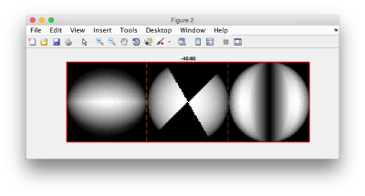
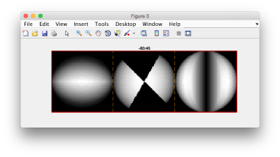
In order to be certain about Dynamo parametrized the missing wedges, you can just create the two versions:
figure;f = dfmask(64,[-45,60]);dslices(f,'x|y|z','j','*');title('-45:60');shg
figure;f = dfmask(64,[-60,45]);dslices(f,'x|y|z','j','*');title('-60:45');shg
and check the results:
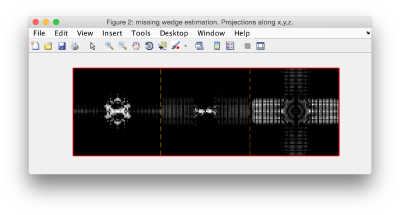
Then you compare it to how a particle of your data set looks like. If myParticle is a random particle out of your tomogram you can write:
dynamo_wedge_estimate(myParticle,'show',1);
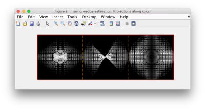
If the visualization does not reveal the structure of the missing wedge because high frequencies are downplayed, you can play with the visualization factors.
dynamo_wedge_estimate(myParticle,'show',1,'factor',0.1);
.
In this case, this data particle should be assigned a couple [-60,45] in columns 14 and 15 of the table.


