Difference between revisions of "Multilevel refinement"
(Created page with "''Dynamo'' computes the angles that produce the maximum correlation in a multilevel fashion. The project parameters <tt>cone_range</tt>, <tt>cone_sampling</tt>, <tt>inplane_r...") |
|||
| Line 3: | Line 3: | ||
== Scanning procedure == | == Scanning procedure == | ||
| + | |||
| + | === Definition of an angular grid == | ||
| + | In Dynamo, an angular grid is defined by five parameters: | ||
| + | ‘cone_range’,’cone_sampling’,’inplane_range’,’inplane_sampling’,’old _angles’ | ||
| + | The first four are project parameters that can be chosen by the user and will be applied for the analysis of all particles. The last one, ‘old_angles’ is obviously different for each particle, and in runtime is read from the table (provided by the user or generated by Dynamo during the iteration procedure). | ||
| + | The ‘cone_’ parameters define a set of orientations that will be sampled around a previously determined old orientation. Here we speak of orientations of the vertical axis of the template, not full unconstrained rotations. Allowing this axis to move inside a cone involves only two Euler angles (tdrot and tilt). ‘cone_range’, is the extent of this cone in degrees (360 being the full possible range of axis orientations). ’cone_sampling’ is the step inside this cone, also in degrees. The orientations are generated so as to provide an uniform coverage. | ||
| + | The ‘inplane_’ parameters complete the set of scanned Euler triplets. After each of the axis reorentations defined by the ‘cone_’ parameters, the template will be rotated about the new orientation of its axis. This involves only the ‘narot’ angle. The project parameter ‘inplane_range’ defines the angular interval to be scanned around the old value of narot, and ‘inplane_sampling’ defines the interval. | ||
| + | By convention, passing equal values to ‘inplane_range’ and ‘inplane_sampling’ generates a grid without ‘inplane’ rotations: only reorientations of the axis will be scanned. | ||
=== Base level scan== | === Base level scan== | ||
| Line 12: | Line 20: | ||
When all the angles in the base level have been scanned, the optimal angles are considered and a new set of angles to scan is defined around these. The geometry of the new set is defined by the angular parameters of the previous level with this formula. | When all the angles in the base level have been scanned, the optimal angles are considered and a new set of angles to scan is defined around these. The geometry of the new set is defined by the angular parameters of the previous level with this formula. | ||
| − | < | + | <nowiki>cone_range[l] = refinem_factor*cone_sampling[i-1]; |
| − | cone_sampling[i] = cone_sampling[i-1]/2;< | + | cone_sampling[i] = cone_sampling[i-1]/2;</nowiki> |
| − | + | ||
| + | The project parameter ‘refine’ defines how many times this process will be repeated for each particle. ‘refine_factor’ defines the range of the new set of angles. A value of 2, for instance, means that the range of the new grid should twice as large as the step of the old grid. | ||
== Visualizing angular distributions == | == Visualizing angular distributions == | ||
You can simulate the method of ''Dynamo'' to compute a multilevel refinement with the command <tt> dynamo_angles_multigrid</tt> | You can simulate the method of ''Dynamo'' to compute a multilevel refinement with the command <tt> dynamo_angles_multigrid</tt> | ||
| − | g=dynamo_angles_multigrid(60,3,45,5,[0, | + | |
| + | <tt>g=dynamo_angles_multigrid(60,3,45,5,[0,45,0],3,2,0,0);</tt> | ||
| + | |||
| + | The output will be a cell array, each entry are the euler triplets at each level. The transition fro one level to the next is in this case generated around the center of the angular grid. Remember that in real applications the finer grid will be centered at the angle that yields the highest similarity. | ||
| + | |||
| + | The output can be shown with <tt>dynamo_plotangles</tt>. This function works for a matrix entry, so that in order to see the different levels, you'll need to iterate it: | ||
| + | |||
| + | <nowiki>for i=1:length(g); | ||
| + | [x,h]=dynamo_plotangles(g{i}); | ||
| + | h.MarkerFaceColor=rand(3,1); | ||
| + | end </nowiki> | ||
| + | |||
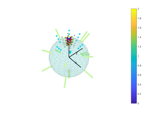
| + | [[File:AngularGridAnglePlot.png|thumb|center|500px|loop on <tt>dynamo_plotangles</tt>]] | ||
== Additional angular parameters == | == Additional angular parameters == | ||
| − | Some other parameters are available | + | Some other parameters are available to define initial scanning orientations: |
| + | * <tt>cone_flip</tt> | ||
| + | * <tt>inplane_flip</tt> | ||
| + | |||
| + | When activated, they extend the basic grid generated by the basic parameters by flipping the original set. For instance, | ||
| + | |||
| + | <tt>g=dynamo_angles_multigrid(60,15,45,5,[0,0,0],0,1,1,0);figure;dynamo_plotangles(g);</tt> | ||
| + | |||
| + | would generate this scanning geometry: | ||
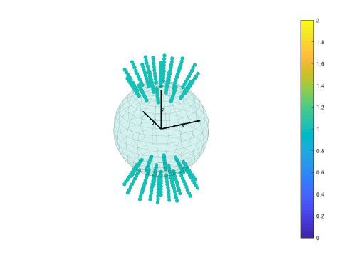
| + | [[ File:AngularGridFlip.png|thumb|center|500px| effect of switching <tt>cone_flip </tt>]] | ||
Revision as of 09:32, 27 October 2017
Dynamo computes the angles that produce the maximum correlation in a multilevel fashion. The project parameters cone_range, cone_sampling, inplane_range and inplane_sampling determine a base level that is scanned exhaustively.
Contents
Scanning procedure
= Definition of an angular grid
In Dynamo, an angular grid is defined by five parameters:
‘cone_range’,’cone_sampling’,’inplane_range’,’inplane_sampling’,’old _angles’ The first four are project parameters that can be chosen by the user and will be applied for the analysis of all particles. The last one, ‘old_angles’ is obviously different for each particle, and in runtime is read from the table (provided by the user or generated by Dynamo during the iteration procedure). The ‘cone_’ parameters define a set of orientations that will be sampled around a previously determined old orientation. Here we speak of orientations of the vertical axis of the template, not full unconstrained rotations. Allowing this axis to move inside a cone involves only two Euler angles (tdrot and tilt). ‘cone_range’, is the extent of this cone in degrees (360 being the full possible range of axis orientations). ’cone_sampling’ is the step inside this cone, also in degrees. The orientations are generated so as to provide an uniform coverage. The ‘inplane_’ parameters complete the set of scanned Euler triplets. After each of the axis reorentations defined by the ‘cone_’ parameters, the template will be rotated about the new orientation of its axis. This involves only the ‘narot’ angle. The project parameter ‘inplane_range’ defines the angular interval to be scanned around the old value of narot, and ‘inplane_sampling’ defines the interval. By convention, passing equal values to ‘inplane_range’ and ‘inplane_sampling’ generates a grid without ‘inplane’ rotations: only reorientations of the axis will be scanned.
= Base level scan
During the scanning procedure, Dynamo will start with a loop on the base level angles. In this loop scans a single angle by computing the full cross correlation matrix between the rotated template and the particle. Then, a shift limiting is applied onto the matrix, and the maximal cc inside the limited ccmatrix is computed. If this maximum is larger than the previously stored maximum for the full set of angles, this angle and the shifts where the cc maximum is located are set as best aligning parameter, and the cc is stored.
The set of angles scanned at this level is regularly distributed (in the space of rotations SO(3)) around the rotation stored for the particle in the previous iteration (which should be stored in the table)
Refinement scan
When all the angles in the base level have been scanned, the optimal angles are considered and a new set of angles to scan is defined around these. The geometry of the new set is defined by the angular parameters of the previous level with this formula.
cone_range[l] = refinem_factor*cone_sampling[i-1];
cone_sampling[i] = cone_sampling[i-1]/2;
The project parameter ‘refine’ defines how many times this process will be repeated for each particle. ‘refine_factor’ defines the range of the new set of angles. A value of 2, for instance, means that the range of the new grid should twice as large as the step of the old grid.
Visualizing angular distributions
You can simulate the method of Dynamo to compute a multilevel refinement with the command dynamo_angles_multigrid
g=dynamo_angles_multigrid(60,3,45,5,[0,45,0],3,2,0,0);
The output will be a cell array, each entry are the euler triplets at each level. The transition fro one level to the next is in this case generated around the center of the angular grid. Remember that in real applications the finer grid will be centered at the angle that yields the highest similarity.
The output can be shown with dynamo_plotangles. This function works for a matrix entry, so that in order to see the different levels, you'll need to iterate it:
for i=1:length(g);
  [x,h]=dynamo_plotangles(g{i});
  h.MarkerFaceColor=rand(3,1);
end
Additional angular parameters
Some other parameters are available to define initial scanning orientations:
- cone_flip
- inplane_flip
When activated, they extend the basic grid generated by the basic parameters by flipping the original set. For instance,
g=dynamo_angles_multigrid(60,15,45,5,[0,0,0],0,1,1,0);figure;dynamo_plotangles(g);
would generate this scanning geometry:

