Walkthrough for template matching

Dynamo includes a set of tools for location of particles inside tomograms. The most simple one is template matching.

Template matching

In this technique, a template representing a molecule of interest is systematically cross-correlated against a tomogram, producing a cross-correlation map of the tomogram. Each pixel in this map represents a score assigned the corresponding pixel in the tomogram map. This score measures the similarity of the neighbourhood of the tomogram pixel to the used template. This similarity is measured exclusively inside a mask.

Data set

Tomogram description

The tomogram contains a buffer with T20S proteasome on a holey carbon grid collected on a Krios + K2. Original pixelsize was 1.76 angstroms. The tomogram provided here has bin binned twice (yielding thus 7.04 ang), defocus is 4.4 microns, no CTF correction, no energy filter.

Acknowledgements

The tomogram has been kindly provided by Alex Noble, from the New York Structural Biology Center. Data collection was performed using Leginon and Appion-Protomo at the Simons Electron Microscopy Center and National Resource for Automated Molecular Microscopy located at the New York Structural Biology Center, supported by grants from the Simons Foundation (349247), NYSTAR, and the NIH National Institute of General Medical Sciences (GM103310) with additional support from Agouron Institute [Grant Number: F00316].

Getting the tomogram

XXXXX

Visualizing the tomogram

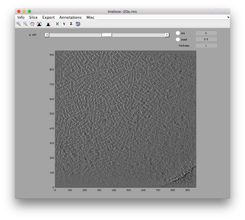
We can get a first glance on how the tomogram looks like:

dtmshow -otf t20s.mrc  

to use the on-the-fly access to the slice shown at each given moment, or

v = dread('t20s.mrc');dtmshow(v); 

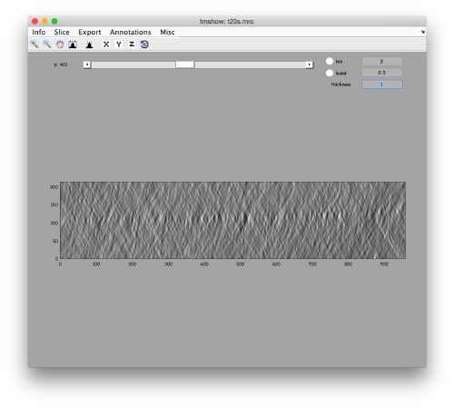
to preload the full tomogram into a memory variable (arbitrarily called v). In either option, you will see, the proteasomes are densely packed in an layer. The layer is slightly oblique, what can be seen browsing through z or y.

dtmshow on the pt20s tomogram, View along z

Navigating on-the-fly you'll see that transitions in y are slower than transitions in z, because all the pixels of the same slice are stored sequentially in the disk.

dtmshow on the pt20s tomogram, View along y

Estimation of the missing wedge

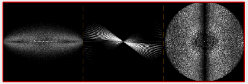
Estimation of the missing wedge'

Creating a template

There are different strategies to create the first template. In the case where the general shape of each protein is roughly recognisable by eye, it is not difficult to just crop and align manually some of the particles. When this is not possible, you have the option of using a density map that mimics the general topology of your protein.

Through manual alignment

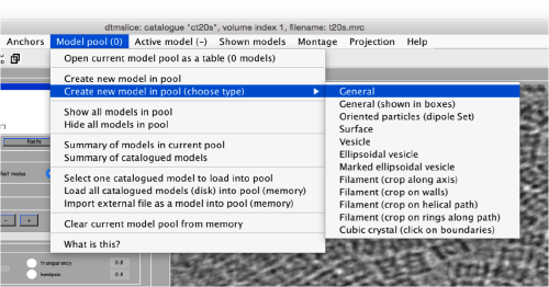
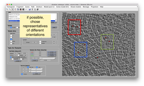
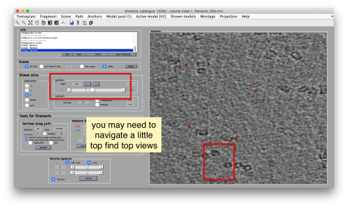
Manual selection of some particles

We use for this our tool dtmslice. As the tomogram is provided is fairly small you can probably just open it without any further binning.

dtmslice t20s.mrc -cc ct20

dtmslice on tomogram

dtmslice on tomogram

Pick particles with the C key

Use the wheel to go up and down in the tomogram to locate top views

Cropping the borders of a template

Template cropped to 32 pixels

Through geometrical shapes

Alternatively, you can use dynamo_mask or dynamo_tube to create a synthetic model.

Creating a cross correlation process

<notwiki>ptm = dynamo_match(fileFull,'average48.em','mask','maskData48.em',....
   'outputFolder','cs30',...
   'ytilt',[-39,36],'sc',[1000,1000,300],'cr',360,'cs',30,'bin',1);<notwiki>

<notwiki>------------------------------------------------------------

Template matching process.
computing in CPU
Output folder: cs30.TM

A total of 1 tiles have been created

 - Mb per tile (reading)   : 724.19
 - Mb per tile (operation) : 663.84
... initializing output elements

Preparing to run on 1 blocks Running on single processor

Computing tile 1
  -Range (original block): x[1:958] y[1:926] z[1:214]
  -Range (binned block)  : x[1:479] y[1:463] z[1:107]
 ... tile 1 finished in 387 seconds (8 for setup;  7.73 per triplet)
 [ok] ... template matching process completed upto creation of cross correlation
      you can proceed to peak location and particle extraction.

---

</notwiki>

The Process object

The return of the function <notwiki>ptm</nowiki> is an object of class XXX. In short, this is an object created

Locating cross correlation peaks

Extracting a table

A table can be extracted through:

myTable = pff.peaks.computeTable('mcc',0.378);

Visual evaluation of results

Looking at cropped particles

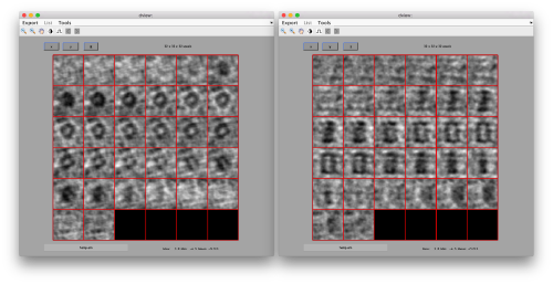
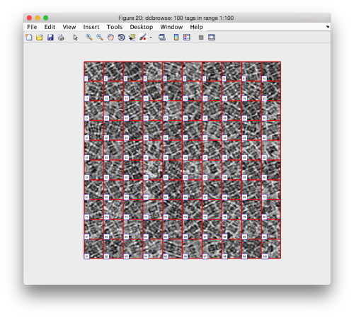
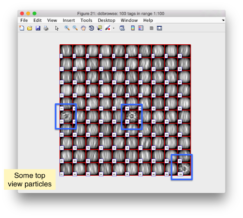
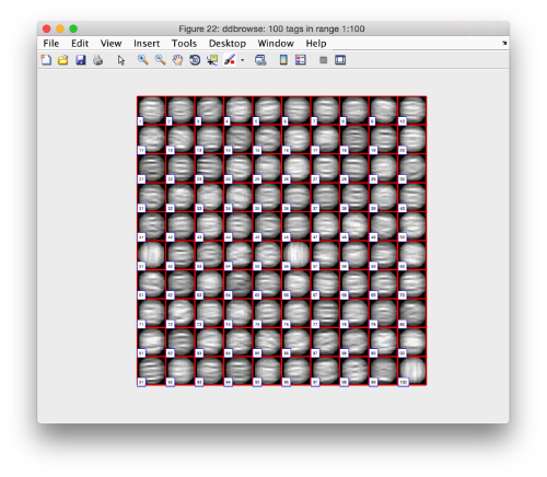
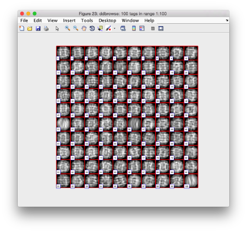
We can check how the individual particles look like on a gallery modus:

pff.peaks.browse();

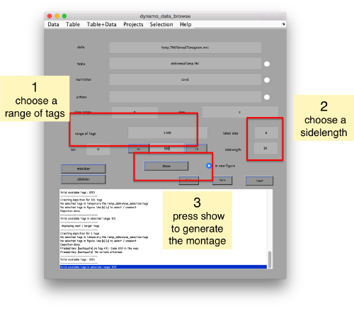
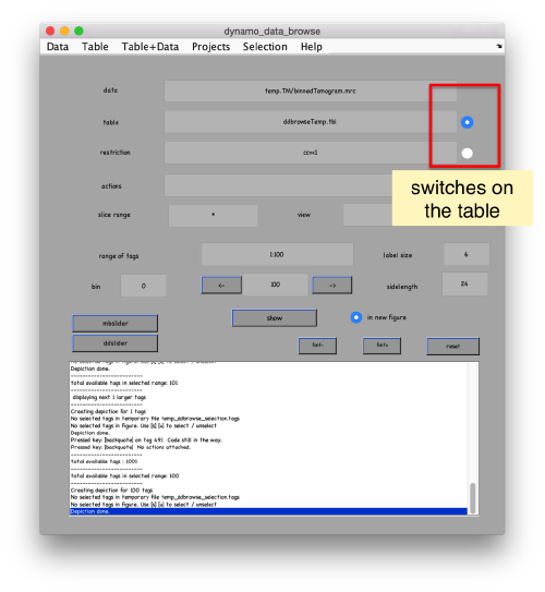
This order just opens ddbrowse. We are using here the support object peaks, but this command is equivalent to just invoking ddbrowse

ddbrowse('d','cr30.TM','t',myTable);

ddbrowse with a tomogram as a data source, needing the input of a sidelength in pixels

Result launched by ddbrowse without a connected table

The table must be connected to align the particles

z-view of aligned particles

x-view of aligned particles

y-view of aligned particles

Looking at averages

o = pff.peaks.average();