Advanced starters guide

This walkthrough uses a small size example based on a real tomogram to covers several tasks.

The example data set

The data is a fraction of a tomogram. The full tomogram was used in "Cryo-electron tomography reveals novel features of a viral RNA replication compartment." (Ertel et al.), and represents several FHV viruses docked in the membrane of a mythocondrion.

Downloading

In principle, you can download all the files related to this example with the command:

 dpkhelp.wiki.downloadExample('fhv');

If it fails under Matlab or the Dynamo command line, you can try to directly use the linux order

wget  https://wiki.dynamo.biozentrum.unibas.ch/w/doc/data/fhv/crop.rec 

or

curl -O  https://wiki.dynamo.biozentrum.unibas.ch/w/doc/data/fhv/crop.rec 

unter MacOS.

This should have created the file called crop.rec in your current directory.

Size check of a file

You're probably curious to see what's inside, so that let's write first:

dfile crop.rec

to let Dynamo check the dimensions of the file. The header of a .rec file is readed as a regular mrc, yielding:

 filetype: volume
 size: 1285 x 956 x 786

So, it's a tomogram.

Lightweight visualization

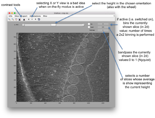
We can inspect quickly its contents with dtmshow

dtmshow -otf crop.rec

Hereby, the flag -otf means "on the fly", telling dtmshow to not preload the full tomogram, but to access in disk the individual slices that are needed when inspecting a particular area.

Basic controls of dtmshow

Go up and down. We want to select the locations were the vesicles intersect the mythocondrion membrane and average them together. For this, we need to catalogue the tomogram, so that our annotations are stored with a clear relationship with the tomogram.

Cataloguing the tomogram

We can create catalogues just to contain a single tomogram. They are useful to keep track of all annotations, and of the typical transforms (binning, cropping of fractions) that we usually perform on a larged size tomogram of interest. In this case, we can create the catalogue directly from the command line:

 >dcm -c create fhv 

where dcm is the short form of dynamo_catalogue_manager and fhv is just an arbitrary name. The just created catalogue is empty, and we can add our tomogram with:

 dcm -c fhv -at crop.rec

We can check that the tomogram is in the catalogue by asking Dynamo to show the contents of the catalogue

dcm -c fhv -l tomograms

or

dcm -c fhv -l t

The flag -l asks Dynamo to list items of a given category of catalogue contents, in this case tomograms

Prebinning the tomograms

We typically want to prebin the tomogram, i.e., have a version of smaller size that is known to the catalogue. This version will be useful in some operations that require a full tomogram in memory, an operation that can consume much memory and need a long time. In this example, this is probably not necessary: a tomogram with a sidelength on x and y of ~1000 pixels shouldn't pose any visualization problem. Still, in the command line, we can write

dynamo_catalogue_bin('fhv', 1, 'zchunk', 300); 

where the parameter zchunk represents the maximum number of z slices that are kept simultaneously in the memory during the binning process. This parameter might be important for larger size tomograms.

Operation with GUI

These steps could have been performed thorugh the dcm GUI <tbi>

Annotation of particle positions

Now we can open the tomogram through the catalogue:

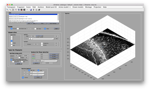
dtmslice crop.rec -c fhv  -prebinned 1 

dtmslice opened on the FHV example tomogramdtmslice

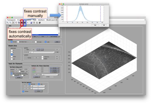
Probably you don't like the initial contrast, change it with the button in the toolbar.

contrast adjustment options inside dtmslice

Navigating the tomogram

Use the bar to move the slice up and dow, or drag it with the cursor while keeping the main mouse button pressed. Other axiliary tools are the keys x,y,z to change the slice orientation, the number of projected slices (called "thickness" in the GUI controls).

Creation of models to contain annotations

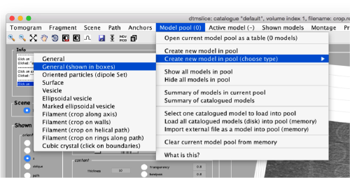
In this example we just want to manually pick some particles. This can be done creating a general or box model, which will reside in memory till we save it into the catalogue.

Creating a new model in the scene. Each annotation is represented by a box

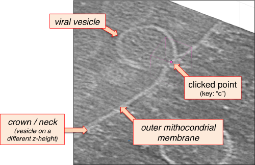
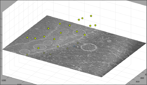
After creating the model, it will be only model currently active in the dtmslice scene. You can add new points pressing on [c]. The idea is to mark on the positions where you see the "neck" of a vesicle (what we called "crowns") in contact with the mythocondrial membrane.

Clicking the crowns on screen

The last marked point can be deleted by pressing [delete]. An arbitrary point can be deleting by clicking on it with the auxiliary mouse button. This will open a menu that includes the option of deleting the point (through Ctrl+X in Linux or Cmmd+X in Mac).

At this stage you probably want to change the transparence of the depicted slice, so that you can control which objects have been already clicked below the depicted slide.

Selection of points. Transparency of slide was set to 0.8

.

When you are done, remember to save the model, using the menu options on active model or simply clicking on the disk icon in tomoslice.

Cropping particles

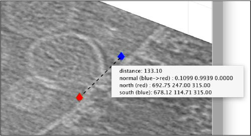
Now we want to use the positions that we have marked to extract the subtomograms and format them as a data folder. The first thing we nee is an estimation of the sidelength in pixels of each of the subtomograms. In dtmslice We can use the keys [1] and [2] to define two anchor points that appear as rombohedra. Clicking (with the right button) onto the black dashed that links the will show on screen both coordinates and the distance between them. All distances are reported in pixels of the not-binned tomogram: even if you are using any un-binned version, Dynamo keeps track of it.

Measuring distances with [1] , [2] and right-click

.

We will thus choose to create a datafolder with a cubic sidelength of 128 pixels (remember that the particles will be cropped in the unbinned tomogram). This will ensure that the crowns fit comfortably inside the physical box, even if our manual picking imposes an error of several pixels. If you were using, say, a thickness parameter of 10 pixles in dtmslice, you have to count with at least this inaccuracy in the location of the particles.

Now, we check that the catalogued tomogram contains the model that we manually picked before:

>> dcmodels fhv
Volume 1 contains 1 models in total
/Users/casdanie//fhv/tomograms/volume_1/models/mboxes.omd

Creating a table

We could just use the catalogue GUI to extract the particles, be it is also possible top roceed directly with the command line. We will use the dtcrop command, .which requires preparing a table with the information of the model.

  m = dread('/Users/casdanie//fhv/tomograms/volume_1/models/mboxes.omd');
t = m.grepTable();

Here, you read the file into a model object (which we arbitrarily choose to call m), and then you use the grepTable method on this object to extract a variable into your workspace. We arbitrarily call it t.

Note that we can extract models directly from the output of dcmodels

  dcmodels fhv -i 1 -ws o;
m = dread(o.files{1});
t = m.grepTable();

i.e., we load the answer of dcmodels for volume index -i 1in the output variable o . Inside it, there is a field called 'files' which contains a cell array of files containing models. Then we read the first entry o.files{1}.

Whichever way you create the table variable t, it is just a matrix with a row for each particle, and a summary of the information coded inside can be created through:

</nowiki>>>dtinfo(t);

       size                :  22 35 
       NaNs                :  0

COLUMN 

[ 2 ] marked for alignment: 22 [ 3 ] included in average : 22 [ 4-6 ] shifts : all zero [ 7-9 ] angles : all zero [ 10 ] cross correlation : min: 0.00 max: 0.00 mean: 0.00 std: 0.00 [ 13 ] Fourier sampling : 1 (single tilt around y) [ 13 ] fsampling types : all of the same type [14-15] ytilt range : min:120.00 max:120.00 [16-17] xtilt range : min:120.00 max:120.00 [ 20 ] linked volumes : total 1 (labels: [1]) [ 21 ] regions inside tomograms : total 1 (labels: [0]) [ 22 ] user-defined classes: total 1 (labels: [0]) [ 23 ] annotation types : total 1 (labels: [0]) [24-26] spatial locations : initialized: 22 [ 24 ] * x : min: 645.21 max: 1001.92 mean: 799.05 std: 109.44 [ 25 ] * y : min: 23.78 max: 917.51 mean: 484.07 std: 271.28 [ 26 ] * z : min: 198.00 max: 563.00 mean: 415.55 std: 114.03 [ 31 ] original tags : total 1 (labels: [0]) [ 32 ] compacted particles : total 1 (labels: [1]) [ 34 ] references : total 1 (labels: [0]) [ 35 ] subreferences : total 1 (labels: [0]) [ 36 ] apix : Warning: column not available in this table [ 37 ] defocus : Warning: column not available in this table</nowiki>

Using dtcrop

The simplest syntax of dtcrop<t/t> requires passing the name of the tomogram from which we want to crop (syntax varies for cropping from multiple tomograms). We know that the file is crop.rec, and we could directly insert this name in the command. But a catalogued model already contains information about its source tomogram (inside its property cvolume, so that we can always track it back. We could then define a variable

tomogramFile = m.cvolume.file();

and launch the cropping order

o = dtcrop(tomogramFile,t,'particlesData',128);

where you could add the mw flag to let Dynamo use several cores. In any case, for this number or particles the cropping should take some seconds. The last part of the final output into screen should look like this:

21 [read_subtomogram] Volume has size 1285 956 786
[read_subtomogram] Accessing subvolume x: 713:840; y: 339:466; z: 160:287  totalling ~ 16.0Mb
Elapsed time is 0.191014 seconds.
22 
Total time invested in cropping: 7s
[table_crop] Done extracting 20 particles
             from tomogram      :"/Users/casdanie/dynamo/devmac/workplace/paris/crop.rec" 
             destination folder :"particlesData" 
             excluded particles : 2   
 
 [ok] table_crop 

informing you that some of the particles where excluded, as they were probably too close to the boundary of the tomogram, given the sidelength we asked for. Inside the created data folder,

you will find the table particlesData/crop.tbl, which only indexes the actually cropped particles.

Creating an average

The particles can now be averaged together. They have different orientations, but in this tomogram we only have a fraction of the membrane.

oa = daverage('particlesData','t','particlesData/crop.tbl');

If you want to let Dynamo pass maps into Chimera, you have to inform Dynamo on the location of Chimera.

dchimera -path /Applications/Chimera.app/Contents/MacOS/chimera 

Creating a project

We first need to create files with the average and the table that we have till now in memory:

dwrite(t,'raw.tbl');
dwrite(oa.average,'rawTemplate.em');

We can create a project directly thorugh the command line:

dcp.new('first','d','particlesData','template.em','rawTemplate.em','masks','defaults','t','particlesData/crop.tbl');

mbparse.multicore.checkPhysicalCores

Your project invokes multicore operations (2 cores required).
Dynamo  will now test your hardware to check that it can run the project.
Starting parallel pool (parpool) using the 'local' profile ...

After running the project, we check the created average.

ddb first:a -v 

Aligning the axis of symmetry

sal = dalign(myParticle,template,'cr',360,'cs',30,'ir',0,'dim',32,'limm',1,'lim',[10,10,10]);