Difference between revisions of "Framework for estimation of membrane thickness"
| Line 51: | Line 51: | ||
</nowiki> | </nowiki> | ||
| − | == Creating | + | == Creating distance filters== |
We first create a set of filters that model the distance between the two layers of the membrane. | We first create a set of filters that model the distance between the two layers of the membrane. | ||
| Line 57: | Line 57: | ||
<tt> t = dpkfw.mdm.templateSeries('size',16,'thickness',1,'distance',[3:7]); </tt> | <tt> t = dpkfw.mdm.templateSeries('size',16,'thickness',1,'distance',[3:7]); </tt> | ||
| − | Here, <tt>t</tt> is a [[cell array]], containing 5 volumes of 16x16x16 pixels each. Each volume contains a "model" of a membrane. | + | Here, <tt>t</tt> is a [[cell array]], containing 5 volumes of 16x16x16 pixels each. Each volume contains a "model" of a membrane. You can visualize them with: |
| + | |||
| + | <tt>figure;dslices(t,'projy','*','dim',[1,5]);</tt> | ||
| + | |||
| + | [[File:MembraneDistanceFilters.png|thumb|center|300px| Y projections of the five filters]] | ||
== Applying the filters onto a particle == | == Applying the filters onto a particle == | ||
Revision as of 11:46, 4 May 2017
This framework is more useful in plastic sections. The premise is that an alignment project has been created to fix the position an orientation of a set of points of interest inside a membrane. In a later stage, we want to get an estimation on the distance between the membrane layers on each particle. This task can be performed through a multireference analysis, but it can also be approached with an analysis a posteriori as sketeched here.
Contents
Reading the particles
The easiest way to bring particles aligned by a project is through the use of the dpkdata.Reader object. If you store the table and data folder of your project in myTable and myData
r = dpkdata.Reader();
r.setSource('table', myTable,'data',myData);
you can access the particles throught the getParticle method:
p = r.getParticle(12,'align',1);
gets the particle with tag 12 as a variable p in the workspace. You can also read all the particles as a matlab cell array through
pa = r.getParticle('*','align',1);
Note that pa may have empty spaces: only the positions with an actual particle tag in the data folder will be occupied. For instance, if you don't have a particle labelled wiht 4 in your data folder, you will see it as.
>> pa

pa  =

  1×194 cell array

  Columns 1 through 5

    [96×96×96 double]    [96×96×96 double]    [96×96×96 double]    []    [96×96×96 double]

  Columns 6 through 9

    [96×96×96 double]    [96×96×96 double]    [96×96×96 double]    [96×96×96 double]
You can create a compact version of this cell array:
pac = mbg.cellCompact(pa);
>> pac

us =

  1×193 cell array

  Columns 1 through 4

    [96×96×96 double]    [96×96×96 double]    [96×96×96 double]    [96×96×96 double]

  Columns 5 through 8

   [96×96×96 double]    [96×96×96 double]    [96×96×96 double]    [96×96×96 double]
Creating distance filters
We first create a set of filters that model the distance between the two layers of the membrane.
t = dpkfw.mdm.templateSeries('size',16,'thickness',1,'distance',[3:7]);
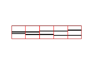
Here, t is a cell array, containing 5 volumes of 16x16x16 pixels each. Each volume contains a "model" of a membrane. You can visualize them with:
figure;dslices(t,'projy','*','dim',[1,5]);
Applying the filters onto a particle
If you have your particle in the Matlab/Dynamo workspace with name p you can type.
o = dpkfw.mdm.bestFilteringDistance(p,'templates',t);
The output structure o contains several fields with different output aspects.
>> o

o =

  output with properties:

        ok: 0
    report: {}
        cc: {[1×1 struct]  [1×1 struct]  [1×1 struct]  [1×1 struct]  [1×1 struct]}
     ccmax: [0.3385 0.3321 0.7576 0.3305 0.3393]
In particular, ccmax is telling you the response of the particle to each filter. In this case, the largest response is to the third filter in t, corresponding to an space of 5 pixels.
Loop on particles and distance histogram
Now you can put all these elements together and compute the largest response for each particle.
for i=1:length(pac)
    o = dpkfw.mdm.bestFilteringDistance(pa{i},'templates',t);
    [maxcc,myIndex] = max(o.ccmax);
    indexList(i) = myIndex(1); % in case there are two maxima
    disp(i);
end
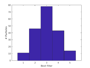
Now, in the position i of numeric array indexList you have the index of the filter in t that responded best to the particle pa{i}. This can be depicted with the hist command in Matlab.
  figure;hist(indexList,[1:5]);
>> xlabel('Best filter');
>> ylabel('# Particles');
You'll need to convert each index to the actual number of pixels of the intermembrane space, and of course to physical units.

