Difference between revisions of "Vesicle models"
(Created page with "Vesicle models are appropriate when particles are evenly distributed on surfaces reasonably similar to spheres or ellipsoids. The model can estimate the center and radius pro...") |
|||
| (22 intermediate revisions by the same user not shown) | |||
| Line 2: | Line 2: | ||
The model can estimate the center and radius provided points provided by the user in the visible part of the object, or the other way round, letting the user provided center and radius. | The model can estimate the center and radius provided points provided by the user in the visible part of the object, or the other way round, letting the user provided center and radius. | ||
| + | ==Important parameters== | ||
| + | ===Radius=== | ||
| + | Given in pixels. | ||
| + | Can be estimated or provided by the user. | ||
| + | |||
| + | ===Center=== | ||
| + | Given in pixels. | ||
| + | Can be estimated or provided by the user. | ||
| + | |||
| + | === Separation === | ||
| + | Given in pixels. | ||
| + | Defines the mean separation of the cropping positions to be defined in the vesicle surface. When choosing this value, you should think on [[Seed oversampling|oversampling]] the actual distribution of particles that you expect. | ||
| + | |||
| + | |||
| + | ==Picking vesicles in a tomogram browser== | ||
| + | |||
| + | There are different methods for vesicle picking interactively, depending on the precision you need. When choosing your method, remember that, if necessary, vesicles can be fitted against the tomogram density map in a later stage. If such a fitting is possible, you don't need to spend too much time trying to make your manual picking too precise, but just reasonable enough to be used as a seed for the automated fitting procedure. | ||
| + | |||
| + | ===Cloud of points=== | ||
| + | |||
| + | The most robust method requires from the user to pick several points in each vesicle model, and then let ''Dynamo'' fit the radius and the center. This procedure can be performed through the browser [[dtmslice | <tt>dtmslice</tt>]], as shown in the next images. | ||
| + | |||
| + | |||
| + | [[File:VesiclePickGlobal.png|thumb|center|500px|A tomogram with several vesicles shown in <tt>dtmslice</tt>]] | ||
| + | |||
| + | First of all we need to define a model of type vesicle into the model pool viewed by <tt>dtmslice</tt>. | ||
| + | |||
| + | [[File:VesicleClickSelectVesicleModelDetail.png|thumb|center|500px|Creation of a vesicle model]] | ||
| + | |||
| + | Once the model is created an active, we can navigate in the tomogram (for instance, by dragging the slice through movement of the cursor while the main mouse button is pressed). Three layers are normally enough. | ||
| + | |||
| + | [[File:VesicleClickSeveralLayers.png|thumb|center|900px|Click vesicle points (in pink) on different ''z'' levels (use [<tt>c</tt>] to pick each)]] | ||
| + | |||
| + | After collecting four of five points on each layer, we can zoom out (with, for instance, <tt>[-] </tt>) and bring the slice to a slower ''z'' value. | ||
| + | |||
| + | [[File:VesicleClickAllLayers.png|thumb|center|500px|View from a lower ''z'' level ]] | ||
| + | |||
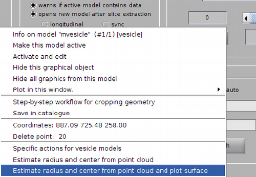
| + | Now, we just need to invoke the method that fits the <tt>center</tt> and <tt>radius</tt> properties of a vesicle given a cloud of points. From the command line, this method is called <tt>approximateGeometryFromPoints</tt>. In the browser <tt>dtmslice</tt> we can invoke it directly by secondary clicking on one of the points of the model and selecting the option for fitting and plotting. | ||
| + | |||
| + | {|style="margin: 0 auto;" | ||
| + | | [[File:VesicleClickMenuFitting.png|thumb|center|500px|Menu options after secondary click on a model point]] | ||
| + | | [[File:VesicleClickMenuFittingDetail.png|thumb|center|500px|Detailed view on the menu options.]] | ||
| + | |} | ||
| + | |||
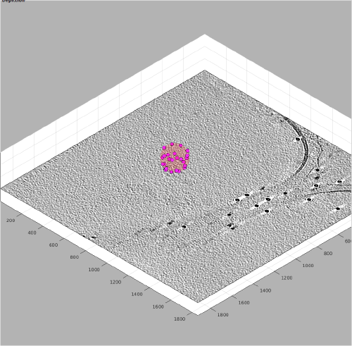
| + | A transparent surface should be visible, allowing you to judge the quality of the fitting quickly sliding the slice up and down. | ||
| + | [[File:VesicleClickFittingInTomoslice.png|thumb|center|500px|Depiction of the fitted vesicle surface]] | ||
| + | |||
| + | === From dipole set models === | ||
| + | It is also possible to use other models to define vesicle models. This is useful when you have several vesicles in one tomogram, and you don't want to initiate a vesicle model for each one of them. The [[dipole set models| dipole set model]] allows creating in a single model several 'dipoles', each one of them having a <tt>center</tt>, a <tt>north</tt> and a <tt>south</tt>. | ||
| + | We can use this model to define each vesicle from a dipole: the <tt>center</tt> property of the dipole can be directly transferred to the vesicle, and the radius of the vesicle can be defined as the distance between the <tt>center</tt> and <tt>north</tt> coordinates registered in the dipole. | ||
| + | |||
| + | You can use this code to convert a dipole set into a set of vesicle models. The code assume that the dipoles set model is in the catalogue, and that the resulting models are also saved into the catalogue. | ||
| + | |||
| + | <nowiki> | ||
| + | % | ||
| + | dipoleSetModelFile = '~/first/tomograms/volume_1/models/dipoleset.omd'; % absolute path to your model | ||
| + | |||
| + | % reads the model | ||
| + | ds = dread(dipoleSetModelFile); | ||
| + | |||
| + | % checks the number of individual dipoles | ||
| + | disp(sprintf('Found %d dipoles in the set',length(ds.dipoles))); | ||
| + | |||
| + | % loops on all the dipoles present in the set | ||
| + | for i=1:length(ds.dipoles); | ||
| + | |||
| + | % selects the i-th individual dipole in the set | ||
| + | dipole = ds.dipoles{i}; | ||
| + | |||
| + | % creates a vesicle model | ||
| + | v = dmodels.vesicle(); | ||
| + | |||
| + | % prepares a name for each individual dipole | ||
| + | v.name = sprintf('%srawVesicle_%d',ds.name,i); | ||
| + | |||
| + | % links the created model with the catalogued volume | ||
| + | % of the dipole set module | ||
| + | v.cvolume = ds.cvolume; | ||
| + | |||
| + | % initiates the vesicle model | ||
| + | v.center = dipole.center; | ||
| + | v.radius = norm(dipole.center - dipole.north); | ||
| + | |||
| + | % saves the model back into the catalogue | ||
| + | v.saveInCatalogue(); | ||
| + | |||
| + | end | ||
| + | </nowiki> | ||
==Command line== | ==Command line== | ||
Here come some examples of creation and manipulation of vesicle models from the command line | Here come some examples of creation and manipulation of vesicle models from the command line | ||
| − | === | + | ===Creation through user points=== |
| − | + | ||
| + | The method is called <tt>approximateGeometryFromPoints</tt>. If a vesicle object <tt>v</tt> has a set of points stored in the <tt>points</tt | ||
| + | > property (i.e., <tt>v.points</tt> contains a matrix of Nx3 numbers, each one a 3d coordinate of the vesicle membrane), invoking the order <tt>v.approximateGeometryFromPoints</tt> will write into <tt>v.radius</tt> and <tt>v.center</tt> the codes estimation for radius and center. | ||
| − | === | + | ===Creation through center and radius=== |
| + | |||
| + | This code merely explains how to create an uniform distribution of points on a vesicle model. The central idea is to define the distance between points with the <tt>separation</tt> property (in pixels), and then invoke the method <tt>updateCrop</tt> that produces the <tt>crop_point</tt> coordinates. | ||
| + | <!--[[File:vesicle_point_distribution_on_example_with_given_radius.png|thumb|right|300px| A screenshot on <tt>dpreview</tt> ]]--> | ||
| + | <nowiki> | ||
a = dmodels.vesicle(); % creates an empty vesicle model | a = dmodels.vesicle(); % creates an empty vesicle model | ||
a.radius = 70; | a.radius = 70; | ||
| Line 20: | Line 114: | ||
axis equal; % for a better visualization, same scale an x,y,z | axis equal; % for a better visualization, same scale an x,y,z | ||
shg | shg | ||
| + | </nowiki> | ||
| + | |||
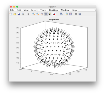
| + | [[File:vesicle_point_distribution_on_example_with_given_radius.png|thumb|center|400px| Table plot of positions and particles generated by a vesicle model]] | ||
| + | |||
| + | ==Fitting vesicles== | ||
| + | |||
| + | === Against tomogram data === | ||
| + | |||
| + | ''Dynamo'' includes some tools for cross correlation based pattern matching. These can be used to fit the center and radius in a roughly picked vesicle. The script that we provide below illustrates how to use the low level vesicle finding utilities in a real life example. | ||
| + | |||
| + | The assumption is that a set of models of approximately picked vesicles (maybe [[Vesicle_models#From_dipole_set_models | converted]] from a [[dipole set models |dipole set]]) has been defined in the tomogram with index 1 of a catalogue located in the folder <tt>'../catalogues/ctfCorrected</tt> with relation to the current directory. The script extracts the models whose name follows a pattern as a [[matlab cell array | cell array]] and then loops on them, fitting them to a simulated vesicle. | ||
| + | |||
| + | The fitting procedure for each vesicle works by first extracting from the tomogram a cube around the vesicle (with {{t| extractEnclosingVolume}}). | ||
| + | Then, the low-level fitting tool is called <tt>dpkfw.vesicle.ccGlobal.locateRadius</tt>, and works by testing a set of predefined radiuses. The radius that yields the largest cross correlation is selected. For each radius, the function computes a global cross correlation between the cropped enclosing volume, thus fitting also the center of the vesicle. | ||
| + | |||
| + | Note that the code below does not overwrite the original models, but manually created a fitted version of each one, which is then saved into the original catalogue. | ||
| + | |||
| + | <nowiki>% extracts model files in a catalogued volume of interest. | ||
| + | files = dynamo_catalogue_models('../catalogues/ctfCorrected','i',1,'nameContains','rawVesicle'); | ||
| + | |||
| + | disp(sprintf('Found %d raw vesicle files in the set',length(files))); | ||
| + | |||
| + | % loops on all the dipoles present in the set | ||
| + | for i=1:length(files); | ||
| + | |||
| + | % | ||
| + | disp(sprintf('Fitting vesicle %d in model file %s',i,files{i})); | ||
| + | |||
| + | % converts the file into a model object | ||
| + | raw = dread(files{i}); | ||
| + | |||
| + | % prepares another vesicle to contain a fitted version of the original | ||
| + | % one. | ||
| + | fitted = copyof(raw); | ||
| + | % this vesicle model is assigend to the same catalogued volume as the | ||
| + | % original model 'raw' | ||
| + | % It also inherits its center and radius properties. | ||
| + | |||
| + | fitted.name = ['fittedVesicle_',num2str(i)]; | ||
| + | |||
| + | |||
| + | % extracts the cube around the estimated center of the vesicle | ||
| + | % As a buffer, we add 30 pixels to the estimated radius | ||
| + | [dataCube,outputEnclosing] = fitted.extractEnclosingVolume('radius',fitted.radius+30); | ||
| + | |||
| + | |||
| + | if isempty(dataCube) | ||
| + | % if the volume went out of scope, we desist on analyzing this vesicle | ||
| + | disp(sprintf('Could not extract data from vesicle %d',i)); | ||
| + | continue; | ||
| + | end | ||
| + | |||
| + | % pixels of the membrane of the vesicle template that | ||
| + | membraneThickness = 10; | ||
| + | |||
| + | % set of radii to be tested | ||
| + | listRadius = fitted.radius-30: fitted.radius+30; | ||
| + | |||
| + | % It's normally convenient to introduce a binning factor | ||
| + | % All magnitudes are rescaled automatically, so that all data | ||
| + | % is expressed in unbinned tompgrams | ||
| + | binningFactor = 2; | ||
| + | |||
| + | % operates the fitting | ||
| + | centering = dpkfw.vesicle.ccGlobal.locateRadius(dataCube,listRadius,.... | ||
| + | 'bin',binningFactor,'membraneThickness',membraneThickness,'bar',true); | ||
| + | |||
| + | |||
| + | % puts the result of the cross correlation back into the vesicle model | ||
| + | fitted.radius = centering.r; | ||
| + | |||
| + | % the output of the extraction operation includes an utility to | ||
| + | % transform coordinates between the extracted enclosing volume and the | ||
| + | % original tomogram | ||
| + | fitted.center = outputEnclosing.dVolume.coords.local2real(centering.center); | ||
| + | |||
| + | % puts the model contanining a fitted vesicle inside the catalogue | ||
| + | fitted.saveInCatalogue(); | ||
| + | |||
| + | end | ||
| + | </nowiki> | ||
Latest revision as of 10:00, 24 February 2017
Vesicle models are appropriate when particles are evenly distributed on surfaces reasonably similar to spheres or ellipsoids. The model can estimate the center and radius provided points provided by the user in the visible part of the object, or the other way round, letting the user provided center and radius.
Contents
Important parameters
Radius
Given in pixels. Can be estimated or provided by the user.
Center
Given in pixels. Can be estimated or provided by the user.
Separation
Given in pixels. Defines the mean separation of the cropping positions to be defined in the vesicle surface. When choosing this value, you should think on oversampling the actual distribution of particles that you expect.
Picking vesicles in a tomogram browser
There are different methods for vesicle picking interactively, depending on the precision you need. When choosing your method, remember that, if necessary, vesicles can be fitted against the tomogram density map in a later stage. If such a fitting is possible, you don't need to spend too much time trying to make your manual picking too precise, but just reasonable enough to be used as a seed for the automated fitting procedure.
Cloud of points
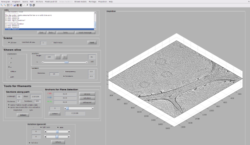
The most robust method requires from the user to pick several points in each vesicle model, and then let Dynamo fit the radius and the center. This procedure can be performed through the browser dtmslice, as shown in the next images.
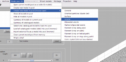
First of all we need to define a model of type vesicle into the model pool viewed by dtmslice.
Once the model is created an active, we can navigate in the tomogram (for instance, by dragging the slice through movement of the cursor while the main mouse button is pressed). Three layers are normally enough.
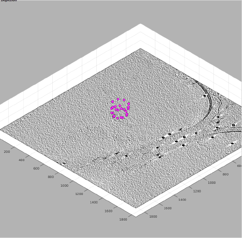
After collecting four of five points on each layer, we can zoom out (with, for instance, [-] ) and bring the slice to a slower z value.
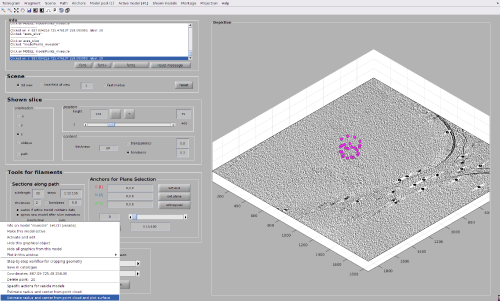
Now, we just need to invoke the method that fits the center and radius properties of a vesicle given a cloud of points. From the command line, this method is called approximateGeometryFromPoints. In the browser dtmslice we can invoke it directly by secondary clicking on one of the points of the model and selecting the option for fitting and plotting.
A transparent surface should be visible, allowing you to judge the quality of the fitting quickly sliding the slice up and down.
From dipole set models
It is also possible to use other models to define vesicle models. This is useful when you have several vesicles in one tomogram, and you don't want to initiate a vesicle model for each one of them. The dipole set model allows creating in a single model several 'dipoles', each one of them having a center, a north and a south. We can use this model to define each vesicle from a dipole: the center property of the dipole can be directly transferred to the vesicle, and the radius of the vesicle can be defined as the distance between the center and north coordinates registered in the dipole.
You can use this code to convert a dipole set into a set of vesicle models. The code assume that the dipoles set model is in the catalogue, and that the resulting models are also saved into the catalogue.
%
dipoleSetModelFile = '~/first/tomograms/volume_1/models/dipoleset.omd'; % absolute path to your model

% reads the model
ds = dread(dipoleSetModelFile);

% checks the number of individual dipoles
disp(sprintf('Found %d dipoles in the set',length(ds.dipoles)));

% loops on all the dipoles present in the set
for i=1:length(ds.dipoles);

    % selects the i-th individual dipole in the set
    dipole = ds.dipoles{i};

    % creates a vesicle model
    v = dmodels.vesicle();

    % prepares a name for each individual dipole
    v.name = sprintf('%srawVesicle_%d',ds.name,i);

    % links the created model with the catalogued volume
    % of the dipole set module
    v.cvolume = ds.cvolume;

    % initiates the vesicle model
    v.center = dipole.center;
    v.radius = norm(dipole.center - dipole.north);

    % saves the model back into the catalogue
    v.saveInCatalogue();

end
Command line
Here come some examples of creation and manipulation of vesicle models from the command line
Creation through user points
The method is called approximateGeometryFromPoints. If a vesicle object v has a set of points stored in the points property (i.e., v.points contains a matrix of Nx3 numbers, each one a 3d coordinate of the vesicle membrane), invoking the order v.approximateGeometryFromPoints will write into v.radius and v.center the codes estimation for radius and center.
Creation through center and radius
This code merely explains how to create an uniform distribution of points on a vesicle model. The central idea is to define the distance between points with the separation property (in pixels), and then invoke the method updateCrop that produces the crop_point coordinates.
a = dmodels.vesicle(); % creates an empty vesicle model
a.radius = 70;
a.center = [40,100,200];
a.separation = 15;
a.updateCrop();  % here it will some time computing the particles.
t=a.grepTable(); % extracts the table
dtplot(t,'profile','oriented_positions'); % scatter plot of images
axis equal; % for a better visualization, same scale an x,y,z
shg
Fitting vesicles
Against tomogram data
Dynamo includes some tools for cross correlation based pattern matching. These can be used to fit the center and radius in a roughly picked vesicle. The script that we provide below illustrates how to use the low level vesicle finding utilities in a real life example.
The assumption is that a set of models of approximately picked vesicles (maybe converted from a dipole set) has been defined in the tomogram with index 1 of a catalogue located in the folder '../catalogues/ctfCorrected with relation to the current directory. The script extracts the models whose name follows a pattern as a cell array and then loops on them, fitting them to a simulated vesicle.
The fitting procedure for each vesicle works by first extracting from the tomogram a cube around the vesicle (with extractEnclosingVolume). Then, the low-level fitting tool is called dpkfw.vesicle.ccGlobal.locateRadius, and works by testing a set of predefined radiuses. The radius that yields the largest cross correlation is selected. For each radius, the function computes a global cross correlation between the cropped enclosing volume, thus fitting also the center of the vesicle.
Note that the code below does not overwrite the original models, but manually created a fitted version of each one, which is then saved into the original catalogue.
% extracts model files in a catalogued volume of interest.
files = dynamo_catalogue_models('../catalogues/ctfCorrected','i',1,'nameContains','rawVesicle');

disp(sprintf('Found %d raw vesicle files in the set',length(files)));

% loops on all the dipoles present in the set
for i=1:length(files);

    %
    disp(sprintf('Fitting vesicle %d in model file %s',i,files{i}));

    % converts the file into  a model object
    raw = dread(files{i});

    % prepares another vesicle to contain a fitted version of the original
    % one.
    fitted = copyof(raw);
    % this vesicle model is assigend to the same catalogued volume as the
    % original model 'raw'
    % It also inherits its center and radius properties.

    fitted.name = ['fittedVesicle_',num2str(i)];


    % extracts the cube around the estimated center of the vesicle
    % As a buffer, we add 30 pixels to the estimated radius
    [dataCube,outputEnclosing] = fitted.extractEnclosingVolume('radius',fitted.radius+30);


    if isempty(dataCube)
         % if the volume went out of scope, we desist on analyzing this vesicle
        disp(sprintf('Could not extract data from vesicle %d',i));
        continue;
    end

    % pixels of the membrane of the vesicle template that
    membraneThickness = 10;

    % set of radii to be tested
    listRadius = fitted.radius-30:  fitted.radius+30;

    % It's normally convenient to introduce a binning factor
    % All magnitudes are rescaled automatically, so that all data
    % is expressed in unbinned tompgrams
    binningFactor = 2;

    % operates the fitting
    centering  = dpkfw.vesicle.ccGlobal.locateRadius(dataCube,listRadius,....
        'bin',binningFactor,'membraneThickness',membraneThickness,'bar',true);


    % puts the result of the cross correlation back into the vesicle model
    fitted.radius = centering.r;

    % the output of the extraction operation includes an utility to
    % transform coordinates between the extracted enclosing volume and the
    % original tomogram
    fitted.center = outputEnclosing.dVolume.coords.local2real(centering.center);

    % puts the model contanining a fitted vesicle inside the catalogue
    fitted.saveInCatalogue();

end
